
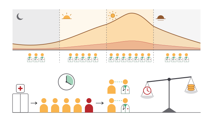
Arrivals follow the clock
Build it: watch the waiting room
- Chart: Queue L (patients waiting) → Chart P[0]
- Statistics: Queue LW (wait of each patient leaving the waiting room) → Statistics P[0]
- Animate on, Start clean; open the Monitor tab and follow single patients


Model codeOpen in Quisim
NumberInput { id:num0; initValue:6; label:"1/λ"; lower:1 }
Wire { from:num0.measureValue; to:rndA.parameterMean }
RandomExponential { id:rndA; seed:42 }
Wire { from:rndA.measureRandomVariate; to:arrive0.parameterDuration }
Arrive { id:arrive0; label:"Entrance" }
Pipe { from:arrive0.outlet; to:queue0.inlet }
Queue { id:queue0; label:"Waiting room" }
Pipe { from:queue0.outlet; to:perform0.inlet }
NumberInput { id:num1; initValue:30; label:"1/µ"; lower:1 }
Wire { from:num1.measureValue; to:rndB.parameterMean }
RandomExponential { id:rndB; seed:77 }
Wire { from:rndB.measureRandomVariate; to:perform0.parameterDuration }
NumberInput { id:num2; initValue:6; label:"Doctors"; lower:1 }
Wire { from:num2.measureValue; to:perform0.parameterCapacity }
Perform { id:perform0; label:"Treatment" }
Pipe { from:perform0.outlet; to:leave0.inlet }
Leave { id:leave0; label:"Discharge" }
Wire { from:queue0.measureLoad; to:chart0.parameters[0] }
Chart { id:chart0; label:"Patients waiting"; height:80; width:300 }
Wire { from:queue0.measureWait; to:stats0.parameters[0] }
Statistics { id:stats0; label:"Mean wait"; height:48; width:128 }Predict: five doctors, exactly enough work?
In your model set Doctors = 5. Work arriving = work the doctors can do.
What happens to the waiting room over the run?
Run it: the queue never settles. It drifts upwards and hardly ever empties again; the mean wait comes out in the hundreds of minutes (about 220 in the run below, against about 18 with six doctors) and keeps growing with the run length: at there is no slack to recover from a busy hour.


Model codeOpen in Quisim
NumberInput { id:num0; initValue:6; label:"1/λ"; lower:1 }
Wire { from:num0.measureValue; to:rndA.parameterMean }
RandomExponential { id:rndA; seed:42 }
Wire { from:rndA.measureRandomVariate; to:arrive0.parameterDuration }
Arrive { id:arrive0; label:"Entrance" }
Pipe { from:arrive0.outlet; to:queue0.inlet }
Queue { id:queue0; label:"Waiting room" }
Pipe { from:queue0.outlet; to:perform0.inlet }
NumberInput { id:num1; initValue:30; label:"1/µ"; lower:1 }
Wire { from:num1.measureValue; to:rndB.parameterMean }
RandomExponential { id:rndB; seed:77 }
Wire { from:rndB.measureRandomVariate; to:perform0.parameterDuration }
NumberInput { id:num2; initValue:5; label:"Doctors"; lower:1 }
Wire { from:num2.measureValue; to:perform0.parameterCapacity }
Perform { id:perform0; label:"Treatment" }
Pipe { from:perform0.outlet; to:leave0.inlet }
Leave { id:leave0; label:"Discharge" }
Wire { from:queue0.measureLoad; to:chart0.parameters[0] }
Chart { id:chart0; label:"Patients waiting"; height:80; width:300 }
Wire { from:queue0.measureWait; to:stats0.parameters[0] }
Statistics { id:stats0; label:"Mean wait"; height:48; width:128 }One shift is an M/M/k queue
Random arrivals (M), random treatment times (M), doctors: open Examples → Erlang C.


Model codeOpen in Quisim
NumberInput { id: numberinput1; initValue:10000; label:"Duration"; width:96; lower:1; upper:1000000; x:22; y:464 }
NumberInput { id: numberinput0; initValue:20; label:"Replications"; width:96; lower:1; upper:100; x:22; y:524 }
Wire { from: numberinput0.measureValue; to: steering0.parameterReplications }
Wire { from: numberinput1.measureValue; to: steering0.parameterDuration }
Steering { id: steering0; replications:20; duration:100000; x:161; y:464 }

NumberInput { id: number0; initValue:125; label:"1/λ\ninterarrival\ntime"; lower:1; x:22; y:48; height:72; width:96 }
NumberInput { id: number1; initValue:100; label:"1/µ\nservice time"; x:22; y:164; lower:1; height:58; width:96 }
NumberInput { id: number2; initValue:1; x:22; y:284; label:"k servers"; lower:1; width:96 }
Wire { from: number0.measureValue; to: function0.parameters[0] }
Wire { from: number1.measureValue; to: function0.parameters[1] }
Wire { from: number2.measureValue; to: function0.parameters[2] }
Function { id: function0; code:"const a = P[1] / P[0], ρ = a / P[2];\nif (ρ >= 0 && ρ < 1) { // Jagerman method\n  let t = 1, s = 1, n = 1;\n  while (n < P[2]) { t *= a / n; s += t; n += 1; }\n  t *= a / n;\n  const Pidle = 1 / (s + t / (1 - ρ)), Pwait = t / (1 - ρ) * Pidle;\n  const Lq = Pwait * ρ / (1 - ρ), Wq = Lq * P[0];\n  M = [ρ, Pwait, Lq, Lq + a, Wq, Wq + P[1], Pidle];\n}\n\n\n\n"; numMeasures:7; numParameters:3; label:"Erlang C"; height:48; width:96; x:162; y:284 }
Number { id: num0; label:"ρ utilization"; width: 156; x:313; y:164 }
Wire { from: function0.measures[0]; to: num0.parameterValue }
Number { id: num1; label:"P(wait) Erlang C"; width: 156; x:313; y:224 }
Wire { from: function0.measures[1]; to: num1.parameterValue }

Number { id: num2; label:"Lq mean queue length"; width: 156; x:313; y:284 }
Wire { from: function0.measures[2]; to: num2.parameterValue }

Number { id: num3; label:"L mean in system"; width: 156; x:313; y:344 }
Wire { from: function0.measures[3]; to: num3.parameterValue }

Number { id: num4; label:"Wq mean wait time"; width: 156; x:313; y:404 }
Wire { from: function0.measures[4]; to: num4.parameterValue }

Number { id: num5; label:"W mean sojourn time"; width: 156; x:313; y:464 }
Wire { from: function0.measures[5]; to: num5.parameterValue }

Number { id: num6; label:"P(idle) idle probability"; width: 156; x:313; y:524 }
Wire { from: function0.measures[6]; to: num6.parameterValue }

Wire { from: number0.measureValue; to: rnd0.parameterMean }
RandomExponential { id:rnd0; x:162; y:48; width:96 }
Wire { from: number1.measureValue; to: rnd1.parameterMean }
RandomExponential { id:rnd1; x:162; y:164; width:96 }
Wire { from:rnd0.measureRandomVariate; to:arrive0.parameterDuration }
Wire { from:rnd1.measureRandomVariate; to:perform0.parameterDuration; bend:-90; incline:100; debend:-100; decline:100 }
Arrive { id:arrive0; x:312; y:48 }
Pipe { from:arrive0.outlet; to:queue0.inlet }
Queue { id:queue0; x:421; y:48 }
Wire { from: queue0.measureLoad; to: chart0.parameters[0] }
Chart { id: chart0; x:502; y:387; label:"Queue length"; height:185; width:421 }
Pipe { from:queue0.outlet; to:perform0.inlet }
Wire { from: number2.measureValue; to: perform0.parameterCapacity; bend:-20; incline:20; decline:-10 }
Perform { id:perform0; x:529; y:48 }
Pipe { from:perform0.outlet; to:leave0.inlet }
Leave { id:leave0; x:631; y:48 }
Statistics { id: statistics1; numParameters:2; warmupWidth:5000; x:503; y:166; label:"Wq Waiting time\n1/µ Service time" }
Wire { from: queue0.measureWait; to: statistics1.parameters[0] }
Wire { from: rnd1.measureRandomVariate; to: statistics1.parameters[1] }
Statistics { id: statistics0; timeAverage:true; numParameters:2; warmupWidth:5000; x:719; y:166; label:"Lq Queue length\nLs=L-Lq Service load" }
Wire { from: queue0.measureLoad; to: statistics0.parameters[0] }
Wire { from: perform0.measureLoad; to: statistics0.parameters[1] }
Statistics { id: statistics2; warmupWidth:5000; x:719; y:28; label:"W Sojourn time"; height:96 }
Wire { from: leave0.measureSojourn; to: statistics2.parameters[0] }
The Function block computes the textbook formulas; the blocks next to it simulate the same queue.
Predict: the afternoon with six doctors
In Erlang C set 1/λ = 6, 1/µ = 30, k servers = 6.
Which share of patients must wait at all? 10%, 30% or 60%?
Run it: , , min. The simulated mean wait (Statistics, 20 replications) comes out at about 19 ± 5 min: the formula's 17.6 lies inside the interval.


Model codeOpen in Quisim
NumberInput { id: numberinput1; initValue:10000; label:"Duration"; width:96; lower:1; upper:1000000; x:22; y:464 }
NumberInput { id: numberinput0; initValue:20; label:"Replications"; width:96; lower:1; upper:100; x:22; y:524 }
Wire { from: numberinput0.measureValue; to: steering0.parameterReplications }
Wire { from: numberinput1.measureValue; to: steering0.parameterDuration }
Steering { id: steering0; replications:20; duration:100000; x:161; y:464 }

NumberInput { id: number0; initValue:6; label:"1/λ\ninterarrival\ntime"; lower:1; x:22; y:48; height:72; width:96 }
NumberInput { id: number1; initValue:30; label:"1/µ\nservice time"; x:22; y:164; lower:1; height:58; width:96 }
NumberInput { id: number2; initValue:6; x:22; y:284; label:"k servers"; lower:1; width:96 }
Wire { from: number0.measureValue; to: function0.parameters[0] }
Wire { from: number1.measureValue; to: function0.parameters[1] }
Wire { from: number2.measureValue; to: function0.parameters[2] }
Function { id: function0; code:"const a = P[1] / P[0], ρ = a / P[2];\nif (ρ >= 0 && ρ < 1) { // Jagerman method\n  let t = 1, s = 1, n = 1;\n  while (n < P[2]) { t *= a / n; s += t; n += 1; }\n  t *= a / n;\n  const Pidle = 1 / (s + t / (1 - ρ)), Pwait = t / (1 - ρ) * Pidle;\n  const Lq = Pwait * ρ / (1 - ρ), Wq = Lq * P[0];\n  M = [ρ, Pwait, Lq, Lq + a, Wq, Wq + P[1], Pidle];\n}\n\n\n\n"; numMeasures:7; numParameters:3; label:"Erlang C"; height:48; width:96; x:162; y:284 }
Number { id: num0; label:"ρ utilization"; width: 156; x:313; y:164 }
Wire { from: function0.measures[0]; to: num0.parameterValue }
Number { id: num1; label:"P(wait) Erlang C"; width: 156; x:313; y:224 }
Wire { from: function0.measures[1]; to: num1.parameterValue }

Number { id: num2; label:"Lq mean queue length"; width: 156; x:313; y:284 }
Wire { from: function0.measures[2]; to: num2.parameterValue }

Number { id: num3; label:"L mean in system"; width: 156; x:313; y:344 }
Wire { from: function0.measures[3]; to: num3.parameterValue }

Number { id: num4; label:"Wq mean wait time"; width: 156; x:313; y:404 }
Wire { from: function0.measures[4]; to: num4.parameterValue }

Number { id: num5; label:"W mean sojourn time"; width: 156; x:313; y:464 }
Wire { from: function0.measures[5]; to: num5.parameterValue }

Number { id: num6; label:"P(idle) idle probability"; width: 156; x:313; y:524 }
Wire { from: function0.measures[6]; to: num6.parameterValue }

Wire { from: number0.measureValue; to: rnd0.parameterMean }
RandomExponential { id:rnd0; x:162; y:48; width:96 }
Wire { from: number1.measureValue; to: rnd1.parameterMean }
RandomExponential { id:rnd1; x:162; y:164; width:96 }
Wire { from:rnd0.measureRandomVariate; to:arrive0.parameterDuration }
Wire { from:rnd1.measureRandomVariate; to:perform0.parameterDuration; bend:-90; incline:100; debend:-100; decline:100 }
Arrive { id:arrive0; x:312; y:48 }
Pipe { from:arrive0.outlet; to:queue0.inlet }
Queue { id:queue0; x:421; y:48 }
Wire { from: queue0.measureLoad; to: chart0.parameters[0] }
Chart { id: chart0; x:502; y:387; label:"Queue length"; height:185; width:421 }
Pipe { from:queue0.outlet; to:perform0.inlet }
Wire { from: number2.measureValue; to: perform0.parameterCapacity; bend:-20; incline:20; decline:-10 }
Perform { id:perform0; x:529; y:48 }
Pipe { from:perform0.outlet; to:leave0.inlet }
Leave { id:leave0; x:631; y:48 }
Statistics { id: statistics1; numParameters:2; warmupWidth:5000; x:503; y:166; label:"Wq Waiting time\n1/µ Service time" }
Wire { from: queue0.measureWait; to: statistics1.parameters[0] }
Wire { from: rnd1.measureRandomVariate; to: statistics1.parameters[1] }
Statistics { id: statistics0; timeAverage:true; numParameters:2; warmupWidth:5000; x:719; y:166; label:"Lq Queue length\nLs=L-Lq Service load" }
Wire { from: queue0.measureLoad; to: statistics0.parameters[0] }
Wire { from: perform0.measureLoad; to: statistics0.parameters[1] }
Statistics { id: statistics2; warmupWidth:5000; x:719; y:28; label:"W Sojourn time"; height:96 }
Wire { from: leave0.measureSojourn; to: statistics2.parameters[0] }The emergency department as blocks


Each patient's wait is recorded; the target is met when 90% of the waits are 20 minutes or less.
Measuring the service level
"At least 90% wait ≤ 20 min" is the same as "the 90% quantile of the wait is ≤ 20 min".


Model codeOpen in Quisim
RandomExponential { id:rndA; mean:6; seed:42; x:22; y:48 }
Wire { from:rndA.measureRandomVariate; to:arrive0.parameterDuration }
Arrive { id:arrive0; label:"Entrance"; x:162; y:48 }
Pipe { from:arrive0.outlet; to:queue0.inlet }
Queue { id:queue0; label:"Waiting room"; x:295; y:48 }
Pipe { from:queue0.outlet; to:perform0.inlet }
RandomExponential { id:rndB; mean:30; seed:77; x:287; y:210 }
Wire { from:rndB.measureRandomVariate; to:perform0.parameterDuration }
Number { id:cap0; value:6; x:440; y:210 }
Wire { from:cap0.measureValue; to:perform0.parameterCapacity }
Perform { id:perform0; label:"Treatment"; x:433; y:48 }
Pipe { from:perform0.outlet; to:leave0.inlet }
Leave { id:leave0; label:"Discharge"; x:570; y:48 }
Wire { from:queue0.measureWait; to:stats0.parameters[0] }
Statistics { id:stats0; x:640; y:100; height:120; width:200; label:"90% wait at most"; warmupWidth:500; quantile:0.9 }
Steering { id:steer0; duration:10500; replications:50; x:22; y:210 }
Statistics with quantile 0.9 on the waits: with 6 doctors, 90% of patients wait at most ≈ 54 ± 7 min (50 replications), far above 20. The quantile and Steering settings need the full version.
The grid search model


Model codeOpen in Quisim
Steering { id:steer0; duration:10500; editions:40 }
Wire { from:steer0.measureEdition; to:grid0.parameters[0] }
Function { id:grid0; label:"Scenario"; numMeasures:2; code:"M = [[30, 10, 6, 15][Math.floor(P[0] / 10)], P[0] % 10 + 1]" }
Wire { from:grid0.measures[0]; to:rndA.parameterMean }
Wire { from:grid0.measures[1]; to:perform0.parameterCapacity }
RandomExponential { id:rndA; seed:42 }
Wire { from:rndA.measureRandomVariate; to:arrive0.parameterDuration }
Arrive { id:arrive0; label:"Entrance" }
Pipe { from:arrive0.outlet; to:queue0.inlet }
Queue { id:queue0; label:"Waiting room" }
Pipe { from:queue0.outlet; to:perform0.inlet }
RandomExponential { id:rndB; mean:30; seed:77 }
Wire { from:rndB.measureRandomVariate; to:perform0.parameterDuration }
Perform { id:perform0; label:"Treatment" }
Pipe { from:perform0.outlet; to:leave0.inlet }
Leave { id:leave0; label:"Discharge" }
Wire { from:grid0.measures[0]; to:stats0.parameters[0] }
Wire { from:grid0.measures[1]; to:stats0.parameters[1] }
Wire { from:queue0.measureWait; to:stats0.parameters[2] }
Statistics { id:stats0; label:"90% wait at most"; warmupWidth:500; numParameters:3; numBatches:10; quantile:0.9; height:120; width:220 }
Function M[0] → arrival mean, M[1] → doctors; both also go to Statistics to label each edition. 1/λ = 6: 6 doctors ≈ 42 ± 22 min, 7 doctors ≈ 18 ± 11 min, 8 doctors ≈ 7 min.
The plan 3/5/7/4 in one model


Model codeOpen in Quisim
Steering { id:steer0; duration:4320; replications:30 }
Arrive { id:shift0; label:"Shift change"; beginAtZero:false; duration:360 }
Pipe { from:shift0.outlet; to:shiftEnd0.inlet }
Leave { id:shiftEnd0 }
Wire { from:shift0.measureNumPassed; to:plan0.parameters[0] }
Function { id:plan0; label:"Staffing plan"; numMeasures:6; code:"const s = P[0] % 4;\nM = [[30, 10, 6, 15][s], [3, 5, 7, 4][s], s == 0, s == 1, s == 2, s == 3]" }
Wire { from:plan0.measures[0]; to:rndA.parameterMean }
Wire { from:plan0.measures[1]; to:perform0.parameterCapacity }
RandomExponential { id:rndA; seed:42 }
Wire { from:rndA.measureRandomVariate; to:arrive0.parameterDuration }
Arrive { id:arrive0; label:"Entrance" }
Pipe { from:arrive0.outlet; to:queue0.inlet }
Queue { id:queue0; label:"Waiting room" }
Pipe { from:queue0.outlet; to:perform0.inlet }
RandomExponential { id:rndB; mean:30; seed:77 }
Wire { from:rndB.measureRandomVariate; to:perform0.parameterDuration }
Perform { id:perform0; label:"Treatment" }
Pipe { from:perform0.outlet; to:leave0.inlet }
Leave { id:leave0; label:"Discharge" }
Wire { from:queue0.measureWait; to:stAll.parameters[0] }
Statistics { id:stAll; quantile:0.9; label:"Whole day"; height:100; width:150 }
Wire { from:queue0.measureWait; to:st0.parameters[0] }
Wire { from:plan0.measures[2]; to:st0.parameterActive }
Statistics { id:st0; quantile:0.9; label:"Night"; height:100; width:150 }
Wire { from:queue0.measureWait; to:st1.parameters[0] }
Wire { from:plan0.measures[3]; to:st1.parameterActive }
Statistics { id:st1; quantile:0.9; label:"Morning"; height:100; width:150 }
Wire { from:queue0.measureWait; to:st2.parameters[0] }
Wire { from:plan0.measures[4]; to:st2.parameterActive }
Statistics { id:st2; quantile:0.9; label:"Afternoon"; height:100; width:150 }
Wire { from:queue0.measureWait; to:st3.parameters[0] }
Wire { from:plan0.measures[5]; to:st3.parameterActive }
Statistics { id:st3; quantile:0.9; label:"Evening"; height:100; width:150 }
Every 360 minutes a "Shift change" event switches arrival mean and number of doctors. M[2…5] switch on the Statistics block of the current shift only (by the time treatment starts). 30 runs of 3 days each.
The extended model: emergency priority


Model codeOpen in Quisim
Number { id: number0; value:15; x:22; y:48 }
Wire { from: number0.measureValue; to: rnd0.parameterMean }
RandomExponential { id:rnd0; seed:88; x:162; y:48 }
Arrive { id:arrive0; label:"Entrance"; x:310; y:48 }
Pipe { from:arrive0.outlet; to:queue0.inlet }
Queue { id:queue0; label:"Waiting room"; x:451; y:48 }
Number { id: number1; value:25; x:20; y:191 }
Wire { from: number1.measureValue; to: rnd1.parameterScale }
Number { id: number2; x:91; y:191; value:2; height:48; width:64 }
Wire { from: number2.measureValue; to: rnd1.parameterShape; bend:-6; incline:-18; debend:-18; decline:-19 }
RandomGamma { id:rnd1; seed:143; x:162; y:191 }
Wire { from:rnd0.measureRandomVariate; to:arrive0.parameterDuration }
Wire { from:rnd1.measureRandomVariate; to:perform0.parameterDuration }
Perform { id:perform0; capacity:4; label:"Treatment"; x:630; y:185 }
Pipe { from:perform0.outlet; to:leave0.inlet }
Leave { id:leave0; label:"Exit"; x:718; y:185 }
Note { id: note0; x:123; y:191; label:"Treatment time" }
Note { id: note1; x:123; y:49; label:"Inter-arrival time" }
Wire { from: queue0.measureWait; to: chart0.parameters[0] }
Chart { id: chart0; x:586; y:7; height:61; width:185; label:"Waiting time" }
Wire { from: queue0.measureWait; to: statistics0.parameters[0] }
Statistics { id: statistics0; x:586; y:96; height:35; width:184; warmupWidth:10000 }
Number { id: number3; value:180; x:22; y:345 }
RandomExponential { id:rnd2; seed:1231; x:162; y:345 }
Arrive { id:arrive1; label:"Emergency entrance"; x:310; y:345 }
Queue { id:queue1; label:"Emergency waiting"; x:451; y:345 }
Function { id: function0; x:540; y:354; code:"M[0] = P[0]>0 ? 1 : 0" }
Wire { from: queue1.measureLoad; to: function0.parameters[0] }
Pipe { from: queue0.outlet; to: select0.inlets[0] }
Wire { from: function0.measures[0]; to: select0.parameters[0] }
Select { id: select0; x:540; y:185 }
Pipe { from: select0.outlet; to: perform0.inlet }
Pipe { from: queue1.outlet; to: select0.inlets[1] }
Note { id: note2; x:123; y:342; label:"Emergency\ninter-arrival time" }
Wire { from: number3.measureValue; to: rnd2.parameterMean }
Pipe { from:arrive1.outlet; to:queue1.inlet }
Wire { from:rnd2.measureRandomVariate; to:arrive1.parameterDuration }
Select takes the emergency queue whenever it is not empty. Extended model