Quisim Simulation Modeling Handbook

Overview

Quisim (https://quisim.com) is a discrete-event simulation tool. A simple graphical user interface allows to create models and run simulations. A specialty is the modeling language of Quisim: It allows to define the simulation model in a declarative way. See the Block API Reference for the complete list of attributes, sockets and defaults.

This handbook is a guide to using the blocks: how a simulation runs, what each block is for, how to build a first model, how to check that it is right, and how to read its results. The exact attributes, sockets and defaults of every block are not repeated here; each block section links to its entry in the Block API Reference, which is generated from Quisim itself.

Why simulate?

Queueing formulas give exact answers only for simple systems such as the M/M/1 or M/M/s queue, and only under strong assumptions:

the system is in equilibrium (steady state),
all distributions are known and do not change over time,
the transient behavior (start-up, peaks, shift changes) is hidden,
only long-run statements are possible, typically as averages.

Discrete-event simulation drops these assumptions. Inter-arrival and service times may follow any distribution, stations may form any network, runs may cover a fixed horizon such as one shift, and you can look at variability as well as at means. For general (G/G/1) queues only complicated approximations exist analytically; a simulation model answers the same question directly (see Beyond M/M/1 below).

How simulation compares with the alternatives:

	Analytical calculation	Discrete-event simulation	Real experiment
Effort for execution	small	middle	large
Effort for modeling	large	middle	large
Effort for analysis	small	middle	large
Time horizon	$\infty$	large	small

A simulation study, step by step

A structured way of working is the recipe for success. Following Banks (1998), a simulation study passes through these steps; the Quisim features that support each step are noted on the right.

Step	What happens	In Quisim
1. Problem formulation	State the problem and the objectives in writing.	—
2. Model conceptualization	Abstract the system's components and their interaction; start simple and grow the model.	From State Diagram to Model
3. Data collection	Identify, specify and collect the data the model needs.	Random Number Blocks: choosing a distribution, input modeling
4. Model translation	Turn the conceptual model into a working simulation.	Blocks and the modeling language
5. Verification	Does the simulation work correctly?	Animation, single step, event list; comparison with M/M/1 theory
6. Validation	Does the simulation correspond to the real system?	Statistics, Report, hypothesis tests
7. Analysis	Interpret the results and develop recommendations.	Steering replications, Statistics confidence intervals, CRN
8. Documentation	Compile the information in line with the study's objectives.	Model file, labels
9. Implementation	Put the decisions into practice.	—

Core Concepts

How a discrete-event simulation runs

A discrete-event simulation computes the system state over time, but the state changes only at discrete, countable points in time, called events. The time between two events of an object is an activity (for example, a service in progress).

An event is a sudden state change at a certain point in time (an arrival, the end of a service).
During an activity the state does not change, so it costs no computation time. This is why discrete-event simulation is efficient compared with continuous simulation.
The event list holds all scheduled events, sorted by time — a "to-do list" of the simulation.

The simulation schedule is a simple loop:

Start: generate the first events.
If the event list is empty or the end time is reached, stop.
Take the next event from the event list.
Set the simulation clock to the time of this event.
Execute the event routine: adjust the system state, schedule new events (at the current time or later), update statistics.
Go to step 2.

Events that happen at the same simulation time must still be processed one after the other, so their order must be well-defined to make runs repeatable. In Quisim you can watch this loop directly: see Quisim Internals > Event List.

Network Structure

A simulation model is represented as a network of connected blocks. The simulation process is determined by process blocks, which are connected via connectors (pipes and wires).

Entity

An entity is an object passed through the simulation's process blocks over time. Processing blocks process entities; their connection in the network determines the path and temporal progression of entities. Entities are represented visually as filled circles by default.

What becomes an entity, what becomes a block? A system is a set of interrelated objects. Objects are permanent or temporary, and stationary or mobile. In a bank, the banker and the counter are permanent and stationary; the customers are temporary and mobile. As a rule:

temporary, mobile objects (customers, parts, orders) become entities;
permanent, stationary objects (counters, machines, staff) become blocks, e.g. a Perform block, whose capacity is the number of parallel staff or machines.

Data that belongs to a single object, such as a customer's arrival time, is kept as an entity attribute (see Entity Attributes). Data that belongs to a resource, such as the number of customers served, is read from the block's measures.

Block Sockets

Simulation blocks have input and output sockets:

Input sockets are always on the left side of a block.
Output sockets are always on the right side of a block.

Two socket types exist:

Entity sockets (green) — for transmitting entities.
Data sockets (silver) — for setting parameters, sending and receiving data.

Example (Queue block): socket I is an input socket for entities, sockets O and R are output sockets for entities. Sockets C and RD set the queue's parameters. Sockets L and LW provide data about the current status of the queue.

In the graphical interface sockets carry short letters (D, N, C, L, …). In the modeling language the same sockets have long names: data inputs are parameters (parameterDuration, parameterCapacity, …), data outputs are measures (measureNumPassed, measureLoad, …), entity sockets are inlet/outlet and a few special names (outRenege, outEvict, inPacket, outPack). The Block API Reference lists both, letter and long name, for every block.

Some blocks have a variable number of sockets. These form a zero-indexed array: P[0], P[1], P[2], … — the first socket is P[0], not P[1]. In the modeling language they are written parameters[i], measures[i], inlets[i] and outlets[i]. The size of each array is set by a count attribute of the block, such as numParameters (Function, Report blocks, Explorer), numOutlets (Decide), numInlets (Select) or numConnectors (Lineup); see Indexed connectors.

Time Units

Quisim time has no fixed unit. All durations (inter-arrival times, service times, renege durations, the Steering duration) are given in model time units. Choose one unit for a model — seconds, minutes, days — and use it consistently. Only the animation speed V of the Steering block is relative to wall-clock milliseconds; for the simulation results only consistency matters. Where an example has a real-world unit, it is stated.

The Modeling Language

Every Quisim model can be written as text. The graphical editor and the text are two views of the same model.

A model has two layers on the same graph:

Entity layer (Pipes): entities flow from an outlet of one block to an inlet of another along a Pipe.
Signal layer (Wires): numeric values flow from a measure (output) of one block to a parameter (input) of another along a Wire.

Each block is written as Type { key: value; key: value }. The id names the block so that pipes and wires can refer to it; other keys set block properties.

Model codeOpen in Quisim

qml

// An M/M/1-type model in the modeling language
RandomExponential { id: rnd0; mean: 50; seed: 88 }   // a value block
Arrive { id: arrive0 }                               // entity blocks
Queue { id: queue0 }
Perform { id: perform0; duration: 40 }               // property set inline
Leave { id: leave0 }

Wire { from: rnd0.measureRandomVariate; to: arrive0.parameterDuration }  // measure -> parameter
Pipe { from: arrive0.outlet; to: queue0.inlet }                          // outlet -> inlet
Pipe { from: queue0.outlet; to: perform0.inlet }
Pipe { from: perform0.outlet; to: leave0.inlet }

Rules worth knowing:

Connections are written as blockId.socketName. Indexed sockets use brackets: decide0.outlets[1], lineup0.inlets[3], function0.parameters[0], function0.measures[0].
A property such as duration: 40 gives the value used when nothing is wired to the matching socket.
Keys like x, y, width, height and label only affect the layout and display.
// starts a comment. Strings may use single or double quotes.
Connections are many-to-many: one outlet may be piped to several inlets and vice versa; one measure may be wired to several parameters. If several wires reach the same parameter, the wire defined last in the code has priority; if several pipes leave the same outlet, the pipe defined last in the code is tried first.
Both the pipe graph and the wire graph may contain cycles (e.g. rework loops).

Getting Started: First Models

This section builds up the first models step by step. Each step adds a block because the previous model needed it.

A minimal model

An Arrive block creates entities; it needs a value for its inter-arrival time D. A Number block provides it. The entity must then go somewhere: an Arrive block has no storage, so an arriving entity must immediately be transported away. A Leave block disposes of it.

Run it in Animation mode with single step and watch one entity every 100 time units pass from Arrive to Leave.

Arrive → Perform: why a Queue is needed

Replace the constant inter-arrival time by an exponential random block, and add a Perform block for the service:

Step through it. When a new entity arrives while the Perform block is busy, the entity cannot leave the Arrive block, and the arrival is blocked until the entity is gone. This delays the next inter-arrival time, so the arrival process is no longer the one you specified: arrivals are delayed instead of waiting in a line. The fix is a Queue in front of the Perform block. The Queue models the waiting line.

The M/M/1 Queue

An M/M/1 queue has

exponentially distributed inter-arrival times (first "M"),
exponentially distributed service times (second "M"),
exactly one server ("1").

Parameters. The random blocks take the mean, which is the inverse of the rate:

arrival block: mean $1/\lambda = 125$ , so the arrival rate is $\lambda = 0.008$ ;
service block: mean $1/\mu = 100$ , so the service rate is $\mu = 0.01$ ;
utilization $\rho = \lambda/\mu = 0.8$ . A steady state exists only if $\lambda < \mu$ .

Expected results (queueing theory, in the same time units):

KPI	Formula	Value
Mean number in system $N$	$\lambda / (\mu - \lambda)$	4
Mean number waiting $N_q$	$\lambda^2 / (\mu(\mu - \lambda))$	3.2
Mean time in system $W$	$1 / (\mu - \lambda)$	500
Mean waiting time $W_q$	$\lambda / (\mu(\mu - \lambda))$	400
Server utilization $\rho$	$\lambda / \mu$	0.8

Verifying the M/M/1 model against theory

A model you can check against theory you already trust is the best first verification exercise. Running this model for 50 000 arrivals gives values that match the formulas closely:

$1/\lambda$	$1/\mu$	$N$ (theory / sim.)	$N_q$ (theory / sim.)	$W$ (theory / sim.)	$W_q$ (theory / sim.)
2	1	1.00 / 1.02	0.50 / 0.52	2.00 / 2.04	1.00 / 1.04
5	1	0.25 / 0.25	0.05 / 0.05	1.25 / 1.24	0.25 / 0.24
5	2	0.67 / 0.66	0.27 / 0.26	3.33 / 3.30	1.33 / 1.30
4	2	1.00 / 1.00	0.50 / 0.49	4.00 / 3.98	2.00 / 1.99

To measure the KPIs in Quisim, wire the block measures into Statistics blocks and run several long replications:

statsNq → $N_q$ (expect 3.2). Queue length is a state that holds for a stretch of time, so it needs the time-weighted average (timeAverage: true).
statsRho → $\rho$ (expect 0.8). The Perform load is 0 (free) or 1 (busy); its time average is the utilization.
statsWq → $W_q$ (expect 400). Waiting times are per-entity observations, so the arithmetic mean (the default) is correct.
statsW → $W$ (expect 500), from the sojourn time (measureSojourn) of entities at the Leave block.

Check that each theoretical value lies inside the reported mean ± confidence radius. If it does not, look for a modeling error, a warm-up that should be cut, or runs that are too short (see Model Testing and Output Analysis).

Beyond M/M/1: G/G/1

A G/G/1 queue has arbitrarily distributed inter-arrival and service times and one server. Only complicated approximations exist for its KPIs (Pollaczek 1930; Kraemer & Langenbach-Belz 1976), but in Quisim you only swap the random blocks. Replace the two exponential blocks by normal distributions truncated at 0, with standard deviation equal to the mean (RandomNormal with mean = std dev = the old mean and lower bound 0). With the same means, waiting changed markedly:

$1/\lambda$	$1/\mu$	$W_q$ M/M/1 (theory)	$W_q$ with truncated normal (simulated)
2	1	1.00	0.40
5	1	0.25	0.09
5	2	1.33	0.52
4	2	2.00	0.78

Same means, different variability, different waiting: this is why the choice of distribution matters (see Random Number Blocks > Choosing a distribution).

Kendall notation in Quisim

Queues are classified as $A/B/c/N^{\max}/K/P$ . Most letters map directly onto a block setting:

Letter	Meaning	Quisim
$A$	inter-arrival time distribution	random block wired to Arrive D
$B$	service time distribution	random block wired to Perform D
$c$	number of parallel servers	Perform capacity C (e.g. capacity 5 for M/M/5)
$N^{\max}$	system capacity	Queue capacity C plus the servers
$K$	size of the arriving population	not a block setting
$P$	queueing discipline	Queue `criterion` and `ascending` (`ascending: false` gives LIFO)

What the blocks do for you

Written by hand, the M/M/1 model needs state variables, an event list and two event routines over the queue length $Q$ and the server state $S$ (free/active):

Arrival of a customer: schedule the next arrival (random inter-arrival time). If $S$ is free, set $S$ to active and schedule the end of service (random service time); otherwise set $Q$ to $Q + 1$ .
End of service: if $Q > 0$ , set $Q$ to $Q - 1$ and schedule the end of service for the next customer; otherwise set $S$ to free.

In Quisim the blocks carry out these routines:

Hand-written model	Quisim
queue length $Q$	`queue.measureLoad`
server state $S$ (free/active = 0/1)	`perform.measureLoad`
"schedule next arrival" with a random inter-arrival time	Arrive pulls a new value from the random block wired to D
"schedule end of service" with a random service time	Perform takes a new duration on each entity's arrival
$Q - 1$ when service ends	the free Perform block pulls the next entity from the Queue (Entity Handover Protocol)
separate random number streams	a separate `seed` on each random block

Block Types

Quisim offers three categories of blocks:

Category	Purpose
Value	Set values, functions, and probability distributions
Entity	Process entities
Report	Display simulation data and provide statistics

The Steering block, which controls the simulation run, is described in its own section, as are the Explorer and BrentOptimize blocks, which run experiments and optimizations across runs.

The sections below explain what each block is for and when to use it. For the complete list of attributes, sockets and defaults, follow the Full reference link of each block to the Block API Reference.

Entity Blocks

Block	Use it to …	Reference
Arrive	create entities at given inter-arrival times	Arrive
Provide	supply entities on demand (unlimited stock)	Provide
Leave	dispose of entities and measure their time in the system	Leave
Perform	model an activity that takes time and capacity	Perform
Queue	let entities wait, with an ordering rule, reneging and eviction	Queue
Decide	route an entity to one of several outlets	Decide
Select	take an entity from one of several inlets	Select
Meter	count passing entities, or let only N pass	Meter
Lineup	synchronize entities from several inlets	Lineup
Pack	pack entities into a packet entity	Pack
Unpack	release the entities of a packet again	Unpack
Set	write an attribute of a passing entity	Set
Get	read an attribute of a passing entity	Get

Arrive Block

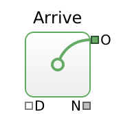
Creates a new entity at output socket O. By default (beginAtZero) the first entity arrives at time 0; otherwise it arrives after the first inter-arrival time. Full reference: Arrive.

To assign a value to the inter-arrival time, set the property to a constant or connect a Value block to socket D.

Note: Arrive has no storage. If a created entity is still present when the next entity arrives, the arrival is blocked until the entity is gone, which delays the next inter-arrival time. Put a Queue after Arrive whenever the next block can be busy. Negative durations are rounded up to 0.

Leave Block

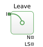
Disposes (removes) an entity from the simulation. It counts the disposed entities (N) and reports the sojourn time of the last exited entity (LS), i.e. the time between its entry into the model and its leave. Full reference: Leave.

Perform Block

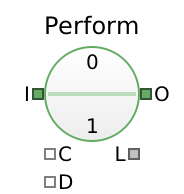
Models an activity with a given delay. Delays any incoming entity by the specified duration, then sends it to output socket O as soon as possible. Has a configurable capacity for parallel entities: set it to inf in the properties panel (capacity: Infinity in the modeling language) for unlimited capacity, which turns the block into a pure delay without resource contention. Full reference: Perform.

The duration D is taken when the entity arrives; negative values are rounded up to 0. A finished entity that cannot be passed on at once keeps occupying capacity while it waits. L counts all entities the block holds: jobs in service, halted jobs (see below) and finished jobs waiting for a blocked outlet.

Excess jobs: two triggers, one action. By default a job, once started, runs to its end. Two attributes can make a running job excess:

haltExcess: a capacity drop. While more jobs run than C allows, the job ranked last is excess. Without haltExcess the capacity is a soft cap: the jobs in service complete as planned, and no new job is accepted until the load has fallen below the new capacity.
preemptive: an arrival that strictly outranks the running job ranked last makes that one job excess (see Preemptive admission below).

Whatever the trigger, an excess job stops processing at once, and the piping of outlet E (outEvict) decides where it goes:

if E is piped and can take it now, it leaves through E; the entity carries its remaining work in the attribute remainingDuration,
otherwise it is halted: it stays in the block (and in L) with its remaining duration frozen. A halted job resumes here as soon as a place in service frees up (best-ranked first), or, if E is piped, leaves through E as soon as E can take entities again.

Finished jobs that wait for a blocked outlet are never touched. With preemptive but without haltExcess, a capacity drop is still a soft cap; only an admitted arrival stops a job, exactly one per arrival.

Ranking. criterion and ascending rank the jobs, as in a Queue: the excess job (victim) is the running job ranked last, halted jobs resume best-ranked first. The criterion remainingDuration (default) is the work still to do (for a halted job its frozen remaining duration), lastEntryTime is the time the job entered the Perform (a resumed job keeps it), and any other value names an entity attribute. The default (remainingDuration, ascending: true) picks the job with the most remaining work; criterion: "lastEntryTime" picks the most recently started job, and ascending: false reverses either rule. Since halting and resuming go by rank, a halted job always ranks below every running job.

Preemptive admission. With preemptive: true a full Perform (load ≥ C) still looks at each offered entity. It ranks the newcomer like a running job: by its full duration D for remainingDuration, by the current time for lastEntryTime, else by its attribute. If the newcomer strictly outranks the running job ranked last, it is admitted and that job is stopped as described above; otherwise the newcomer stays upstream, e.g. in a Queue. The inlet counts as blocked only if no running job could be preempted, e.g. when all places hold finished jobs waiting for a blocked outlet, or C = 0. The criterion decides the discipline:

`criterion`, `ascending`	Newcomer preempts	Discipline
`remainingDuration`, true (default)	if its D is shorter than the longest remaining work in service	shortest remaining processing time first (SRPT)
`lastEntryTime`, `false`	always (it is the latest), stopping the earliest started job	preemptive LIFO (with C = 1)
attribute, true / `false`	if its value is strictly lower / higher than the worst running job's	preemptive priority
`lastEntryTime`, true	never (it would rank last itself)	no preemption

D is read once per job. With preemptive and remainingDuration, D is read already when the job is first offered, to rank it, and the same value is used when it is admitted later (unless it has moved to another block meanwhile); otherwise D is read on arrival as usual.

Outlet E is shown only if haltExcess or preemptive is set, or E is piped; it is then the second outlet. Quisim warns when loading a model in which E is piped but neither haltExcess nor preemptive is set, because then no job will leave through E. A job that left through E can be finished elsewhere, e.g. by another Perform whose duration a Get block reads from remainingDuration.

Preemptive priority example — C = 2 servers shared by high-priority (priority 0) and low-priority (priority 1) jobs. A high-priority job that finds both servers busy with at least one low-priority job interrupts it; the interrupted job is halted (E is not piped) and resumes with its remaining work when a server frees up (preemptive-resume). The Queue in front serves high-priority jobs first, so it always offers the best-ranked waiting job:

Equal priorities never preempt each other. With criterion: "remainingDuration" instead (and no Set blocks), the same model serves by shortest remaining processing time. Piping E, e.g. to a second Perform, lets interrupted jobs leave instead of waiting. The older way with two Perform blocks is shown in Preemptive priority with two Perform blocks under Complete Model Examples.

Queue Block

Stores incoming entities up to capacity C and sends them to the outlet as soon as possible. Full reference: Queue.

If the outlet is blocked and the renege duration RD since the entity's arrival has passed, the entity is sent to output socket R (outRenege) instead. RD is taken on the entity's arrival.

The ordering is set by criterion and ascending. The default criterion lastEntryTime is a keyword for arrival order, not an entity attribute; any other value names an entity attribute (e.g. one written by a Set block) whose numeric value orders the queue. With the default ascending: true the queue is FIFO; ascending: false gives LIFO.

The complete M/M/1 model is shown in Getting Started > The M/M/1 Queue.

Capacity: soft cap or eviction. A full Queue (load = C) accepts no further entity; the newcomer stays upstream, e.g. in the Arrive block, which then tries its next pipe. This holds also when the outlet looks open but the next block refuses the head entity (a Decide used as a gate, a preemptive Perform, a pushing-out Queue): the Queue never admits beyond C. Only an empty Queue passes an entity straight through, and then only if the next block takes it. With C = 0 that is all a Queue does: it is a pure pass-through, and an entity that the next block does not take immediately stays upstream. So a capacity of 0 closes a Queue only when the block behind it is busy or closed as well.

As in a Perform, two attributes act on excess entities, with outlet E (outEvict) as the only way out. A queue has nothing to halt, so without a pipe from E, or while E is blocked, nobody is removed.

evictExcess: a capacity drop. If C is lowered below the current load by a wire, the Queue evicts one entity after another through E until load ≤ C. If E is blocked, it stops and continues as soon as E can take entities again. Without evictExcess C is a soft cap: nobody is removed, the queue just accepts nothing until it has drained below C.
preemptive: an arrival. When the queue is exactly full, a newcomer that would be served before the current victim pushes it out: the victim leaves through E and the newcomer takes its place. Otherwise, or if E cannot take the victim, the newcomer stays upstream. evictExcess alone never pushes out an entity on arrival.

The victim is always the entity that would be served last ("served-last rule"):

Ordering	Served first	Victim (served last)	With `preemptive`, a newcomer at a full queue pushes out the victim
FIFO (`lastEntryTime`, ascending)	earliest arrival	latest arrival	never (it would be served last itself)
LIFO (`lastEntryTime`, `ascending: false`)	latest arrival	earliest arrival	always
attribute, ascending	lowest value	highest value	if its value is strictly lower than the victim's
attribute, `ascending: false`	highest value	lowest value	if its value is strictly higher than the victim's

Each evicted entity gets lastWait like a reneging one. A victim other than the one served last can be modeled with a Decide after the outlet, see Evicting the entity served first under Complete Model Examples.

Outlets O, R and E. Outlet R is shown only if reneging is enabled (renegeDuration finite or RD connected) or R is piped; outlet E only if evictExcess or preemptive is set, or E is piped. The visible outlets are numbered in this order, so E is the second outlet of a Queue without reneging. In the modeling language the names outRenege and outEvict never change. When a model is loaded, Quisim warns if evictExcess or preemptive is set but E is not piped (no entity will be evicted), or if E is piped but neither is set.

LIFO example:

Reneging example — entities that wait longer than 500 time units leave through outRenege:

More patterns built on capacity and eviction are in Complete Model Examples: Line jockeying, Preemptive priority with two Perform blocks and Evicting the entity served first.

Decide Block

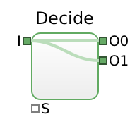
Routes an incoming entity to outlet Os, where s is determined by the value of selection parameter S using round-down logic:

0 ≤ S < 1 → sent to O0
1 ≤ S < 2 → sent to O1
etc.

The number of outlets is set with numOutlets; the outlets are outlets[0], outlets[1], … Wire the selector to decide0.parameterSelectedOutlet. Full reference: Decide.

Pitfall: With nothing connected to S, the default −1 applies and no entity is routed: the block acts as a closed gate and entities stay upstream (typically in a Queue). This is also the intended way to model a gate. The block is also blocked if all outlets are blocked.

Recipe: route to outlet 1 with probability $p$ . Wire a RandomUniform with lower = $p$ and upper = $1 + p$ to S. Then $P[U \ge 1] = p$ , so the entity goes to O1 with probability $p$ and to O0 otherwise. For example, RandomUniform { lower:0.1; upper:1.1 } sends 10% of the entities to O1 (e.g. rework). If $p$ must change during the run, compute lower and upper in a Function block and wire them to the RandomUniform's parameterLower and parameterUpper; keep $p \le 1$ (e.g. with Math.min).

Select Block

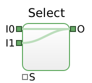
The inverse of Decide: takes an entity from input number s (determined by selection parameter S) and sends it to output socket O. The same round-down logic as Decide applies. The number of inputs is set with numInlets; the inputs are inlets[0], inlets[1], … An inlet is blocked if it is not selected or the outlet is blocked. As with Decide, the default S = −1 selects no input. Full reference: Select.

Meter Block

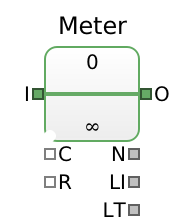
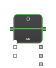
Counts the number of entities passing from input socket I to output socket O. If a capacity is set, the meter stops passing entities when that load is reached. Without a capacity it only counts; with capacity C it closes after C entities until it is reset via R (changing R to a non-zero value resets the count; a constant non-zero value resets it only once). Besides the count N since the last reset, it reports the time when the last entity passed (LT) and the interval between the last two passing entities (LI). Full reference: Meter.

Typical uses: count the parts produced by one machine (place the Meter after the machine, not at the queue entry); release exactly N jobs from a Provide block (Provide → Meter { capacity: N }, see Flow Shop); preload a queue with a given number of entities; record the completion time of the last job via LT.

Lineup Block

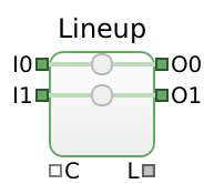
Waits until neededEntities have arrived at distinct inlets (entities "line up"), then sends all of them out simultaneously, each on its corresponding outlet. Full reference: Lineup.

Constraint: 1 ≤ neededEntities ≤ numConnectors. Default: neededEntities = numConnectors.

Pack Block

Packs entities arriving at input socket I into a newly created packet entity arriving from input socket P. The packet entity is sent to outlet O as soon as possible. Full reference: Pack.

The sufficiency B (sufficiency) and capacity C (capacity) are the lower and upper limit of entities to pack. By default B equals C, so Pack { capacity:4 } sends the packet as soon as 4 entities are packed. The packet entity (the container) must be supplied at inPacket, typically from a Provide block; without it, nothing is packed.

Unpack Block

Unpacks a packet entity arriving at input socket I. The inner entities are enqueued and sent one by one to the outlet. The empty packet entity is sent to outlet P (outPack) only after all inner entities have left. Full reference: Unpack.

The inner entities wait as in a Queue: if one cannot be forwarded within the renege duration RD, it is sent to R (outRenege). As in a Queue, R is shown only if reneging is enabled or R is piped, so P is the second or third outlet.

Unpack takes a new packet only when it is empty, and it reads its capacity C only when a packet arrives: it unpacks at most C inner entities, the others stay in the packet and leave with it through P. A later change of C has no effect on the current packet, and Unpack has no outlet E. The measure LD is the time the last exited entity spent packed, from its enqueuing in the Pack block until it left here.

Provide Block

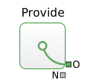
Provisions a new entity at outlet O at any time (on demand). A new entity is created as soon as the previous one has been taken away, so Provide represents an unlimited supply: the bottleneck is always downstream, and no Queue is needed after it. Full reference: Provide.

Set Block

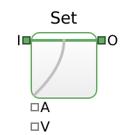
Sets an attribute of a passing entity to a specified value. You may choose any attribute name, but the read-only attributes number and innerEntitiesLength cannot be set. A typical use is to give an entity a type in addition to its number, or to store a value drawn at arrival so that it can be used later. Full reference: Set.

Get Block

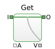
Retrieves the value of an attribute from an entity being evaluated for passing through, and makes it available on the signal layer (e.g. for a Function that drives a Decide block). Full reference: Get.

Example (Set + Get) — each customer draws its service time on arrival, carries it as attribute duration, the Queue serves the shortest one first (criterion: "duration", ascending), and the Perform block uses it:

Entity Attributes

In addition to custom attributes set via the Set block, entities carry built-in attributes: a unique, read-only number, the color and symbol they are drawn with, and the read-only innerEntitiesLength of a packet. Some blocks write an attribute when an entity passes, for example Queue writes lastWait, Perform lastDuration, and a Perform that evicts a job writes its remainingDuration; such values can be read later with a Get block. The Monitor/Entities tab shows the attributes of the entities in the selected block. The complete list, with the block that sets each attribute, is in Entity Attributes of the Block API Reference.

lastEntryTime, the default ordering criterion of Queue and Pack, is a keyword for arrival order, not an entity attribute.

Value Blocks

Block	Use it to …	Reference
Number	provide a constant value	Number
NumberInput	provide a value that can be edited while the simulation runs	NumberInput
Random…	draw random variates from a distribution	Random Number Blocks
Function	compute values with JavaScript code	Function
Aggregate	reduce a stream of values, e.g. to a running sum	Aggregate
Note	put a text note on the canvas	Note

Number Block

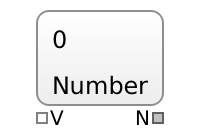
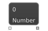
Provides a constant value that can be entered in the properties panel; it can also be set from outside through its input V. Full reference: Number.

Random Number Blocks

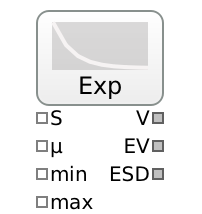
Replace the Number block with one of these stochastic value blocks when inter-arrival or service times are not constant. Each time a connected block pulls a value (e.g. Arrive asking for its next inter-arrival time), a new random number is drawn. Full reference: RandomExponential, RandomGamma, RandomWeibull, RandomUniform, RandomNormal, RandomLognormal, RandomPoisson, RandomDiscrete, ContinuousDistribution, RandomPiecewiseLinear.

Block (GUI)	Modeling language	Distribution
Exp	`RandomExponential`	Exponential
Gamma	`RandomGamma`	Gamma
Weibull	`RandomWeibull`	Weibull
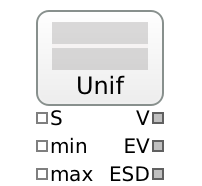
Unif	`RandomUniform`	Uniform
Normal	`RandomNormal`	Normal
Lognorm	`RandomLognormal`	Log-normal
Poisson	`RandomPoisson`	Poisson
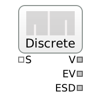
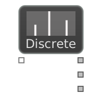
Discrete	`RandomDiscrete`	Discrete (finite set of outcomes)
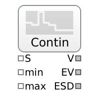
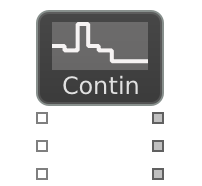
Contin	`ContinuousDistribution`	Empirical continuous (from raw data or a histogram)
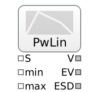
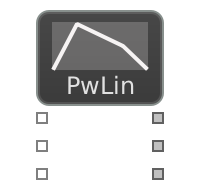
PwLin	`RandomPiecewiseLinear`	Piecewise linear density (generalizes triangular)

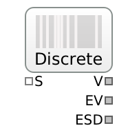
Every random block has a seed input S. With seed 0 (the default) the block draws from the global generator, whose seed is set in the Steering block; a non-zero seed gives the block its own stream. Besides the random variate V, each block outputs the expected value EV and expected standard deviation ESD of the configured distribution. The expected mean and variance are also shown in the properties tab — a quick check that a parameterization gives what you intended.

Exp block specifically: generates exponentially distributed random numbers in the range [min, max]. Its mean µ is 1/rate, and its mean is also its standard deviation. For an M/M/1 queue with arrival rate $\lambda$ and service rate $\mu$ , set the arrival block's mean to $1/\lambda$ and the service block's mean to $1/\mu$ .

Unif block note: range is [min, max) (half-open interval).

Lognorm block note: mean µ and stddev σ are $\mu$ and $\sigma$ on the log scale, so the median is $\exp(\mu)$ , not $\mu$ .

Discrete block note: set probabilities: [0.2, 0.5, 0.3] (weights, normalized by their sum) and optionally values: [1, 5, 10] of the same length; without values the outcomes are $0, 1, \ldots, n-1$ . Both are lists in the properties tab, not wireable inputs.

Contin block note: set values: [3.1, 4.7, 5.2, 8.0] to the raw measurements, in any order. The cumulative distribution is linear between the sorted values and every gap gets the same probability (Law & Kelton), so draws never leave [smallest, largest value]. To let draws fall outside the observed range, add an extra support point to the values (Banks et al.), e.g. values: [0, 3.1, 4.7, 5.2, 8.0] lets durations fall below the smallest observation. For grouped data also set frequencies: then values: [0, 5, 10, 20] are the bin edges and frequencies: [0.3, 0.5, 0.2] give one frequency per bin; draws are uniform within each bin. In both cases min/max truncate the distribution like for the other blocks.

PwLin block note: set values: [0, 1, 3, 4] to the points and densities: [0, 2, 1, 0] to the density at each point; the density is linear in between and normalized by the total area, so only the shape matters. The triangular distribution with minimum $a$ , mode $c$ and maximum $b$ is values: [a, c, b], densities: [0, 1, 0]. A repeated value is a jump of the density, e.g. values: [0, 1, 1, 2], densities: [1, 1, 3, 3] is a step. min/max cut the density at the bounds.

Truncation: all distributions with lower/upper bounds support truncation. Truncation can shift the mean; compare EV with your target.

Prefer bounded distributions for durations. A simulation model should avoid distributions with unbounded support. RandomNormal, RandomLognormal, RandomGamma and RandomWeibull default to min = $-\infty$ ; a negative duration is rounded up to 0 by Arrive and Perform, which puts extra probability on 0 and biases the mean. Set min (at least 0) and, where physically meaningful, max.

Choosing a distribution

Understanding the process behind the data tells you which distribution to try first:

Process	Distribution	Quisim block
Time between independent arrivals; memoryless remaining duration	Exponential (rate $\lambda = 1/\mathrm{mean}$ )	`RandomExponential`
Number of independent events in a fixed interval (e.g. customers per hour)	Poisson (estimate: the sample mean)	`RandomPoisson`
Duration that is the sum of several sub-steps	Normal (truncated at 0), or Erlang/Gamma (an Erlang is a sum of exponentials; Gamma generalizes it)	`RandomNormal` with min 0, `RandomGamma`
Quantity that is the product of factors	Log-normal	`RandomLognormal`
Time until a defect or failure	Weibull (generalizes the exponential)	`RandomWeibull`
Only lower and upper limits are known	Uniform	`RandomUniform`
Minimum, most likely and maximum value are known (expert estimate)	Triangular, or any piecewise linear density	`RandomPiecewiseLinear` with `values: [min, mode, max]`, `densities: [0, 1, 0]`
Finite set of outcomes with known probabilities (e.g. batch size, routing class)	Discrete (estimate: the relative frequencies)	`RandomDiscrete` with `probabilities: [...]`, `values: [...]`
Measured data that no standard distribution fits	Empirical continuous (the data itself)	`ContinuousDistribution` with `values: [...]`, plus `frequencies` for a histogram

The exponential distribution suits inter-arrival times, but because its standard deviation equals its mean it is often too variable for service or treatment times. A Gamma distribution with shape $k > 1$ has less relative variability. Its mean is $k \cdot \theta$ and its variance $k \cdot \theta^2$ , so $k = \mathrm{mean}^2/\mathrm{variance}$ and $\theta = \mathrm{variance}/\mathrm{mean}$ . Example: $k = 2$ , $\theta = 25$ gives mean 50.

Input modeling: from data to parameters

Collect data. About 100 to 200 observations with two to three significant digits. Plan the measurement, evaluate data while collecting, and watch for:
- homogeneity of measurement series (combine only homogeneous series; check with a t-test),
- censored data (artificially extended times, unrecorded long times),
- dependence between variables and on time of day or day of week,
- autocorrelation in seemingly independent observations,
- the difference between input data (not controllable) and output data (what you want to improve).
Identify candidate distributions. Start with a histogram, shortlist candidates (e.g. Pearson or Cullen & Frey plots), and draw QQ plots.
Estimate parameters from the data.
Test the fit with a goodness-of-fit test ( $\chi^2$ test, Kolmogorov–Smirnov test). If it fails, go back to step 2.
Check in Quisim. Compare the block's EV and ESD with the sample mean and standard deviation, and look at the generated values with a Histogram (see Report Blocks).

If no standard distribution fits, two alternatives exist: replay the measured values directly in their original order, or draw repeatedly at random (with replacement) from the measured values (an empirical distribution). Both need representative and long series of measurements; otherwise the same values repeat too often.

When data is missing

Machine specifications: e.g. a printer that delivers 20 pages per minute needs 3 s per page on average.
Standard times in production: MTM (bottom-up, predefined times for manual tasks) or REFA (top-down).
Expert estimates: ask for an optimistic and a pessimistic value, or a variability indication, rather than a single number.
Physical limits: typing speed, walking speed — useful for setting min and max.

Using measured values directly. If you have measurements but no standard distribution fits them, give the measured values to a Discrete or Contin block instead of estimating parameters.

Durations and other continuous quantities: Contin block (ContinuousDistribution). Enter the raw measurements as values, unsorted. The block interpolates between them, so it also draws values in the gaps between observations:

Draws stay within the smallest and largest measured value. If longer or shorter durations are possible, add a bound you believe in, e.g. values: [3, 4.2, 5.1, …, 7.3, 10]. If the data only exists as a frequency table, enter the class limits as values and the counts as frequencies, e.g. 12 jobs of 0–5 min, 30 of 5–10 min and 8 of 10–20 min:

Counts and categories: Discrete block (RandomDiscrete). For batch sizes, number of items per order or the routing class, count how often each outcome was observed and enter the counts as probabilities; they are normalized by their sum. Example: 40 orders with 1 item, 25 with 2 and 15 with 5:

Drawing from the measured values with replacement: the Discrete block with the measurements as values and the weight 1 for each of them draws only values that were actually measured, never values in between. Use it when only the measured values can occur; otherwise prefer the Contin block.

Both blocks can only reproduce what was measured: with few observations, rare long durations are missing and the variability is underestimated. Compare EV and ESD in the properties tab with the sample mean and standard deviation. For raw data the Contin block's EV is close to, but not exactly, the sample mean, because the smallest and largest value get only half the weight of the others.

Time-dependent arrival rates

Real arrival rates change over time: a clinic is quiet at night and busy in the morning. Such arrivals form a non-homogeneous Poisson process with a rate $\lambda(t)$ that depends on the time $t$ . There are two ways to model it in Quisim. The examples use minutes as the time unit and a day of 1440 minutes, with $\lambda = 1/60$ (one arrival per hour) outside 9:00–17:00 and $\lambda = 1/2$ (one every two minutes) inside it.

Approximation: an Exp block with a time-dependent mean. Compute the mean $\mu(t) = 1/\lambda(t)$ from the simulation time T of the Steering block and wire it to the Exp block's µ:

This is simple, but it is only approximately right. Each inter-arrival time is drawn with the mean that is valid when the gap begins, and that gap is not shortened or lengthened when the rate changes during it. The resulting error depends on the direction of the change:

Rate rises (quiet → busy): the arrivals lag behind. The gap that is running at 9:00 was drawn with mean 60. Because the exponential is memoryless, it still has 60 minutes left on average, so the first busy-period arrival comes about an hour late. About $60 \cdot \tfrac{1}{2} = 30$ of the 240 arrivals expected between 9:00 and 17:00 are lost every day, and the morning queue builds up too slowly.
Rate falls (busy → quiet): the error is small. The gap running at 17:00 was drawn with mean 2, so the model produces about one extra arrival.

The approximation is good when the mean $\mu$ is short compared to the time over which $\lambda(t)$ changes noticeably. It is poor for sudden changes and for long quiet periods.

Exact: thinning (Lewis & Shedler, 1979). Choose an upper bound $\lambda_{\max} \ge \lambda(t)$ for all $t$ . Generate candidate arrivals at the constant rate $\lambda_{\max}$ , and keep a candidate arriving at time $t$ with probability $\lambda(t)/\lambda_{\max}$ ; reject the others. The kept arrivals form exactly the non-homogeneous Poisson process with rate $\lambda(t)$ . Because the candidate gaps are short (mean $1/\lambda_{\max}$ ), no change in the rate is skipped.

In Quisim, the acceptance step is the Decide recipe route to outlet 1 with probability $p$ (see Decide Block) with $p = \lambda(t)/\lambda_{\max}$ computed from the simulation time:

Points to watch:

$\lambda_{\max}$ must be an upper bound. If $\lambda(t)$ exceeds $\lambda_{\max}$ , then $p > 1$ , every candidate is accepted, and the model silently produces too few arrivals at the peak. Capping $p$ with Math.min(1, …) hides this error rather than fixing it; choose a larger $\lambda_{\max}$ instead.
Cost: every rejected candidate is a wasted event. Here 720 candidates per day give about 256 arrivals; in the quiet hours only 1 in 30 is kept. If $\lambda_{\max}$ is far above the typical rate, the model runs slower but stays exact.
Count after the Decide. The Arrive block's count N includes the rejected candidates. Measure the arrivals at the accepting outlet (e.g. with a Meter block), and do not set entity attributes before the Decide.

	Exp with time-dependent mean	Thinning
Result	Approximate; arrivals lag behind rate increases	Exact for any $\lambda(t)$
Needs	$\mu(t)$ at the current time	$\lambda(t)$ at the current time and a bound $\lambda_{\max}$
Extra blocks	Function	Function, RandomUniform, Decide, Leave
Good choice when	$\mu$ is short compared to how fast $\lambda(t)$ changes	$\lambda(t)$ changes suddenly or quiet periods are long

Function Block

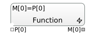
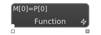
Calls JavaScript function code provided in the properties panel. Uses input parameter array P and writes results to output array M. Statements are separated by ; (semicolon) or by line breaks. Local variables can be declared with let, and a whole array may be assigned to M, e.g. let p=0.5*P[0]/10000; M=[p, 1+p]. All JavaScript Math functions are available. Full reference: Function.

Use context for code evaluated once when the model is loaded (global functions and variables) and init for code evaluated at the start of each simulation run (to reset globals).

The Function is evaluated when one of its first numParameters inputs changes and when one of its outputs is read (immediately, or as a scheduled event with deferredEvaluation). Further inputs added with numRequested or numConsumed do not trigger an evaluation.

Example (adds and subtracts two parameters):

Math Methods

Expression	Meaning
`Math.sqrt(a)`	$\sqrt a$ if $a\ge0$
`Math.exp(a)`	$\mathrm{e}^a$
`Math.pow(a, b)`	$a^b$
`Math.log(a)`	$\ln(a)$ if $a>0$
`Math.log10(a)`	$\log_{10}(a)$ if $a>0$
`Math.sin(a)`	$\sin(a)$
`Math.abs(a)`	$\lvert a\rvert$
`Math.floor(a)`	$\lfloor a\rfloor$
`Math.ceil(a)`	$\lceil a\rceil$
`Math.round(a)`	nearest integer; halves round up toward $+\infty$ , i.e. $\lfloor a + 0.5\rfloor$
`Math.max(a, b)`	$\max\{a, b\}$
`Math.min(a, b, c)`	$\min\{a, b, c\}$

Example — Euclidean distance from $(x, y)$ to $(0, 0)$ :

Ternary (Conditional) Operator

a ? b : c

If logical expression a is true, use b; otherwise use c.

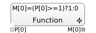
Example — Set M[0] to 1 if P[0] ≥ 1, else 0:

Logical Operators

Operator	Meaning
`x < y`	x less than y
`x <= y`	x less than or equal to y
`x > y`	x greater than y
`x >= y`	x greater than or equal to y
`x == y`	x equal to y
`x != y`	x not equal to y
`(u) && (v)`	both u and v are true
`(u) \|\| (v)`	at least one of u, v is true

Arrays

Arrays are created with [a, b, ...]. Elements are accessed by zero-based index. See also the Array documentation in the Mozilla JavaScript Reference.

Example — look up a value from a fixed list:

P[0] = 0 gives 10, P[0] = 1 gives 15, and so on. P[0] must be an integer index from 0 to 4; a non-integer or out-of-range index gives undefined, so use Math.floor(P[0]) if the index comes from a random block. A typical use is an order quantity per article number, e.g. M[0]=[10,20,15,30,50][P[0]].

Useful array methods (given A = [10,15,15,30,40]):

Method	Result
`A.indexOf(15)`	1 (first index of 15; −1 if not found)
`A.lastIndexOf(15)`	2 (last index of 15; −1 if not found)
`A.some(n => n>20)`	true (at least one element > 20)
`A.every(n => n>20)`	false (not all elements > 20)
`A.find(n => n>20)`	30 (first element > 20)
`A.findIndex(n => n>20)`	3 (index of first element > 20)

Aggregate Block

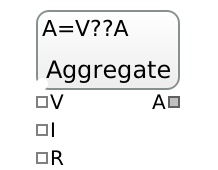
Reduces incoming values to one aggregate value A. The reduction is given as code; for example, a running sum is A+=V with init 0. The default code A=V??A keeps the last value. Each change of the input V triggers the computation, and changing the reset input R to a non-zero value resets A to its init value. Full reference: Aggregate.

Report Blocks

Report blocks show what a model produces. They are also the way to look at the values of a random variable:

Chart displays the values over time,
Histogram displays their distribution,
Report lists them in a table,
Statistics computes means and confidence intervals,
SummaryStatistics estimates a mean and confidence interval from results such as batch means,
EnsemblePlot averages them across replications to find the warm-up.

Block	Use it to …	Reference
Chart	follow values over time	Chart
Histogram	see the distribution of values	Histogram
Report	list values in a table for export	Report
Statistics	estimate means with confidence intervals	Statistics
SummaryStatistics	estimate a mean with confidence interval from results, e.g. Statistics batch means	SummaryStatistics
EnsemblePlot	identify the warm-up phase (Welch plot)	EnsemblePlot

All report blocks have an active input (parameterActive, default: true): data is recorded only while it is true.

Chart Block

Generates a stairstep line chart from provided values; each input is drawn in a different color. Zoom in to see the exact value changes. By default the series of earlier runs are kept; set clearBetweenReplications or clearBetweenEditions to start afresh with each replication or edition. Full reference: Chart.

Example — queue length and server load of an M/M/5 system:

Histogram Block

Draws a histogram. The number of classes is chosen automatically unless numBuckets is set. For levels such as a queue length, set timeAverage so that each value is weighted by the time it holds. Full reference: Histogram.

Example — distribution of queue length and server load of an M/M/5 system, time-weighted:

Report Block

Generates a table with columns: ed (edition), rep (replication), p (input socket), time, v (value). The table can be copied as CSV/TSV with the copy button, e.g. for a hypothesis test in another tool. Full reference: Report.

Example — protocol of queue length and server load of an M/M/5 system:

Statistics Block

Generates statistical calculations from provided values. For each input it outputs the last mean (measures[i]) and the last mean of means (measures[numParameters+i], label MM[i]). Full reference: Statistics.

By default the block computes the arithmetic mean. Set timeAverage for continuous-time state variables like queue length to get the time-weighted average instead (see Output Analysis > Which mean?). Set cumulative for counters such as leave0.measureNumPassed: the statistic is then the difference between end and start values, i.e. the number passed per run (throughput), averaged over replications.

The half-width is reported at the 1 − confidence Student-t level: confidence is the tail probability $\alpha$ , so the default 0.05 gives a 95% interval. Observations from the transient phase are excluded by setting warmupWidth; with warmupMSER the MSER-5 rule chooses the warmup automatically once the simulation has run and writes it into warmupWidth. To get an interval from a single long run, split it into batches with numBatches (batch means). Further options — warm-up and batch widths as record counts instead of simulation times, a correction for correlated batches, per-batch quantiles instead of means — are described in the full reference.

warmupWidth and batchWidth were formerly named warmupDuration and batchDuration.

The last row of the statistics table shows the mean and 1 − confidence confidence radius across all replications. How to read it is explained in Output Analysis > Reading the confidence interval.

What flowed during the run is what the wired blocks received: a recalculation after the run, after a setting changed or warmupMSER wrote its warmup, only updates the Statistics block's own table and measures; run again to pass the new results on.

Cumulative property example

leave0.measureNumPassed is a counter: it reports the running total of entities that have left so far. Its plain mean would average these running totals, which gives about half the final count and has no useful meaning. With cumulative: true the block reports the difference between the end and start values instead, i.e. the number of entities that left during the run. The last row then shows the mean of this count over the 5 replications.

Setting quantile: 1 instead of cumulative: true gives the same result here: the counter starts at 0 in each replication and only grows, so its maximum is the final count. If both are set, quantile takes precedence.

SummaryStatistics Block

Estimates the mean and confidence interval of a sample of results. Every value arriving at its input is one observation: there is no time weighting, warmup or batching. It is the estimation stage after a Statistics block, which does the batching: wire the batch means M[i] of a Statistics into it, directly or through a Function that derives a result from each batch mean. Full reference: SummaryStatistics.

The estimate is computed exactly as Statistics computes its mean of means: per replication the mean of its values, then the Student-t interval over the replications (with a single replication, over its values). Fed with M[0] directly, it shows the same mean and interval as the Statistics' MM[0]. Its measures are the mean, the half-width, the lower and upper limits, the standard deviation of the replication means and the number of values used. With quantile set (in [0,1]), it also outputs that quantile of the replication means (of the values with a single replication) per edition, without a confidence interval.

Do not wire M[i] into another Statistics block: it would batch the results again by time and close its replications in an undefined order with the source.

Its results are set at the end of an edition, together with the Statistics' MM, so an optimizer can use its mean as objective. A recalculation after the run only updates the recalculating block's own view, not the blocks wired to it: a changed confidence, ar1Correction or quantile here, or batch means that change after the run, such as those of a Statistics with warmupMSER, which picks its warmup at the end of the first run; SummaryStatistics then keeps the run's estimate, and running again updates it.

Example — number of entities in an M/M/1 system ( $\rho = 0.8$ ). The Statistics block batches the time-averaged queue length and server load, 10 batches per run. Per batch, a Function adds the two batch means to get the number in the system, and SummaryStatistics estimates its mean and confidence interval over the 5 replications. The theoretical value is $\rho/(1-\rho) = 4$ . Set deferredEvaluation on the Function: both batch means change at the same time, and an immediate evaluation would pass one extra sum per batch with a stale input.

EnsemblePlot Block

Plots the Welch ensemble-averaged time series of the given input parameters P, used to identify the warm-up (transient) phase visually before steady state. Needs multiple replications to be meaningful — about 5 or more is typical. Full reference: EnsemblePlot.

Across replications, each input is ensemble-averaged by observation index ( $\bar{Y}_j = (1/R) \sum_i Y_{ij}$ ) and then smoothed with a moving average. The warm-up duration is read off where the smoothed curve flattens.

As with Statistics, leave timeAverage off for per-event observations like waiting times, and turn it on for continuous-time state variables like queue length. If the curve is too noisy, average more observations per plot point (batchWidth) or widen the moving average (windowWidth, kept below ¼ of the number of plot points); by default a dashed line also marks the MSER-5 truncation point. All settings can be changed after the simulation has finished — the plot re-derives from retained raw data without rerunning the model.

Relation to Statistics: EnsemblePlot (a Welch plot) helps you find the warmup visually; once identified, set warmupWidth on the Statistics block to exclude it from the means and confidence intervals. For a fully automated equivalent, set the Statistics block's warmupMSER attribute — it evaluates MSER-5 on raw observations and writes the suggestion into warmupWidth.

Example — Welch plot of queue length and server load of an M/M/5 system over 5 replications:

Steering Block

Configures simulation-level settings: duration, number of editions and replications, global seed, and simulation speed. Also displays the current virtual time, edition, and replication number. Setting its active input to false halts the simulation. Full reference: Steering.

Since a simulation is stochastic, a single run gives only one possible outcome. Replicate each scenario several times to get stable results and confidence intervals; this is what the replications setting is for.

In replication $r$ ( $r = 0, 1, \ldots, R - 1$ ), every random number stream is reseeded with seed + $r$ : the global stream with the Steering seed, and each random block with its own seed. Replications therefore differ from each other but are reproducible. The edition number does not enter the seed: each new edition starts again at replication 0 with the same seeds, so all editions see the same random numbers. Editions that vary a parameter are thus compared under common random numbers automatically, but repeating an unchanged model in several editions gives identical results. Total number of runs = $E \times R$ . If no global seed is set, the current time is used as the seed.

Recording one value per run: for a measure that only grows, such as a completion time or a counter, set quantile: 1 on the Statistics block. Each replication then contributes its maximum, which is the final value, e.g. the completion time of the last order (see Flow Shop). To record how much a counter grew during the run instead, use cumulative: true.

Experiment and Optimization Blocks

These blocks drive a series of runs: Explorer runs scripted experiments, BrentOptimize searches for the parameter value that optimizes an objective.

Block	Use it to …	Reference
Explorer	script a series of experiments	Explorer
BrentOptimize	find the parameter value that minimizes (or maximizes) an objective	BrentOptimize

Explorer Block

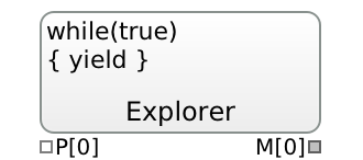
Runs experiments in a loop: its code configures a run through the outputs M, starts it with yield, and reads the results through the inputs P when the run has finished. yield returns true unless the last experiment is done. Default code: while(true) { yield }. Full reference: Explorer.

BrentOptimize Block

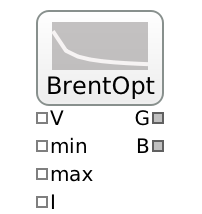
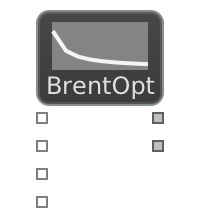
Optimizes an objective locally in the range [lower, upper] using Brent's algorithm. The current guess is adapted each time a new run starts; the first guess is init, if given, otherwise the golden-section point $\mathrm{lower} + 0.382 \cdot (\mathrm{upper} - \mathrm{lower})$ . Wire the objective to V; G outputs the current guess and B the best guess found. Set minimize to false to maximize instead. Full reference: BrentOptimize.

Output Analysis

Terminating vs. non-terminating simulations

Decide first which kind of study you run; it determines the Steering duration and whether a warm-up is removed.

Terminating — the system has a natural end (end of shift, store closing, the last of 20 orders finished). Results refer to the whole run. Set the Steering duration to that horizon (or let the run end with the last event), do not remove a warm-up, and use replications for the confidence interval.
Non-terminating — no natural end; you want steady-state values (e.g. to compare with the M/M/1 formulas). Use a long duration, find the warm-up with EnsemblePlot (≥ 5 replications) or warmupMSER, cut it with warmupWidth, and use replications or numBatches for the confidence interval.

The warm-up can be handled in three ways: simulate longer, start with meaningful initial values (e.g. preload the queue to its steady-state mean with a Meter block), or cut off the warm-up period.

Which mean? Time-weighted vs. arithmetic

A state such as a queue length holds a value for a stretch of time. Its arithmetic mean over the change points is wrong, because it ignores how long each value held. The time-weighted mean is

\hat{\theta}=\frac{1}{t_n-t_1}\sum_{i=1}^{n-1}w(t_i)\left(t_{i+1}-t_i\right),

where the last value $w(t_n)$ does not contribute. Durations of individual entities (waiting times, times in system) are separate observations; their arithmetic mean is correct.

Measure	Kind	Statistics setting
`queue0.measureLoad` (queue length)	state	`timeAverage: true`
`perform0.measureLoad` (busy servers; utilization = average / capacity)	state	`timeAverage: true`
`pack0.measureHasPackage`, `unpack0.measureHasPackage`	state	`timeAverage: true`
`queue0.measureWait` (waiting time)	per-entity duration	`timeAverage: false` (default)
`leave0.measureSojourn` (time in system)	per-entity duration	`timeAverage: false` (default)
`leave0.measureNumPassed`, `arrive0.measureNumPassed` (counters)	count per run	`cumulative: true`

Reading the confidence interval

From $m$ replications (or batches) with means $\hat\theta_1,\dots,\hat\theta_m$ , the Statistics block reports their average $\hat\Theta$ and the confidence radius

\delta = t_{m-1,\,\alpha/2}\cdot\sqrt{S_m^2/m},\qquad S_m^2=\frac{1}{m-1}\sum_{i=1}^m (\hat{\theta}_i - \hat{\Theta})^2,

with $\alpha$ = confidence. The interval $(\hat\Theta-\delta,\hat\Theta+\delta)$ is the result.

The 95% describes the procedure: about 95 of 100 such intervals cover the true mean. It does not mean that this particular interval contains it with probability 95%.
The radius shrinks like $1/\sqrt{m}$ (replications) and like $1/\sqrt{n}$ (observations per run). Halving it takes four times as many replications.
A single replication with numBatches: 1 gives no interval.
Two scenarios whose intervals overlap are not shown to differ significantly. For a sharper comparison, see System Comparison with Common Random Numbers.

Model Testing: Verification and Validation

Decision makers need to know whether a model and its results are correct. Verification asks: does the Quisim model do what the conceptual model says? Validation asks: does the model represent the real system well enough for its purpose? Both are iterative, run throughout model development, and are carried out to the degree the model's intended purpose requires.

Verification checklist

Step through it. Run in Animation mode with single step and watch the event list (Monitor/Events tab) and the entity attributes (Monitor/Entities tab). Typical faults: a missing Queue in front of a Perform block (blocked arrivals), entities stuck in a Pack or Lineup, a Decide with nothing wired to S (closed gate), or a Decide that routes everything to one outlet.
Trace a value over time. Wire the measure of interest (e.g. queue0.measureLoad, or a Get block's measureValue) into a Chart for its history or into a Report for a table you can export.
Check against analytics. Rebuild a known special case, such as the M/M/1 queue, and confirm that the confidence intervals contain the theoretical values (Getting Started > Verifying the M/M/1 model against theory).
Check reasonableness under varied inputs. Push key parameters to extremes (very low or very high load, capacity 1 or $\infty$ ) and check that the outputs move in the expected direction.

Validation in three steps (Naylor, 1967)

Face validity. People who know the real system watch the animation and judge whether it is a reasonable imitation. A weak test, but valuable early on.
Model assumptions. Structural assumptions: how does the system operate (e.g. do two servers work in parallel, or in series)? Data assumptions: are the fitted distributions right? Check them with goodness-of-fit tests (Kolmogorov–Smirnov, $\chi^2$ ) and look for outliers.
Input-output transformation. Feed the model the observed inputs (e.g. the actual arrival times) and compare its output with the real system's output for the same period, using a hypothesis test.

Testing the model against the system

Test $H_0$ : model measure = system measure with a t-test over $n$ independent replications. With the replication average $\bar{y}$ , its standard deviation $\sigma_y$ and the observed system value $\mu_y$ :

t_0 = \frac{\bar y - \mu_y}{\sigma_y/\sqrt{n}},\qquad p = 2\,(1-T(|t_0|, n-1)).

If $p < \alpha$ , reject $H_0$ : the model output differs significantly from the system, and the model needs adjustment. If $p \ge \alpha$ , the data give no evidence against the model. More replications and longer runs both increase the power of the test.

To get one value per replication out of Quisim, either wire the KPI into a Report block and copy the table (columns ed, rep, v), or, for a measure that only grows, use a Statistics block with quantile: 1, which takes the final value of each replication. The test itself can be run in Python:

python

import math
import statistics
from scipy.stats import t
def calc(samples, mu0):
  t0 = (statistics.mean(samples)-mu0) / (statistics.stdev(samples) / math.sqrt(len(samples)))
  p = 2*(1-t.cdf(abs(t0), len(samples)-1))
  return p

From State Diagram to Model

A UML state diagram is a good intermediate step between a problem description and a block network. It consists of states (a phase or condition of an object), events (signals or changes in the environment), transitions (arrows, optionally labeled with the triggering event, a guard condition and an action) and actions (entry, do and exit actions of a state). The entity that runs through the Quisim model plays the role of the object whose states are described.

State diagram element	Quisim
State that lasts a given time (e.g. "Machine Working")	Perform block; `capacity: Infinity` if many entities can be in the state at once
State in which entities wait for a resource	Queue in front of the Perform block
Initial state	Provide → Meter `{ capacity: N }` to inject exactly N entities
Final state	Leave
Transition with a deterministic guard (e.g. "after 10 000 time units")	Decide driven by a Function, e.g. `M[0]=P[0]<10000?0:1`
Transition with a probability	Decide driven by a RandomUniform on $[p, 1+p]$ (see Decide Block)
State memory, such as accumulated working time	Entity attribute, updated with Get → Function → Set
"Number of entities in state X"	`measureLoad` of the corresponding Perform or Queue, wired into a Function

Example: a machine. A machine works for 1000 time units, then goes into maintenance for 100 time units, and back to work; after a total of 10 000 time units it is disposed of. In Quisim, one entity (Provide → Meter {capacity:1}) carries an attribute time, set to 0 at the start. After "Working" and after "Maintenance" a Get → Function → Set chain adds the duration to time. A Decide block, driven by a Function M[0]=P[0]<10000?0:1 on the updated time, either loops the entity back to the work queue or sends it to Leave ("Dispose"). Verify such a model by single-stepping and by wiring the Get block's measureValue into a Report. The complete model and its probabilistic variant are in Examples: Machine State Diagram.

Complete Model Examples

M/M/1 Queue

See Getting Started > The M/M/1 Queue for the model, its expected results, and a version with statistics for verification.

Call Center (Selecting a Queue with Decide)

A call center with regular customers (10 employees) and premium customers (2 employees), in a 10:1 ratio. All customers have exponentially distributed inter-call times (mean 75 s) and call durations (mean 500 s). Time unit: seconds.

Why not two separate queues? Since the two customer types do not interfere, an M/M/10 queue for regular and an M/M/2 queue for premium customers is tempting. But the given data describe only the joint call stream: it is unclear whether the inter-call times of each type are exponentially distributed, so they cannot be derived separately. Instead, the model generates the joint arrival stream and splits it.

Where each parameter goes:

call durations ( $1/\mu = 500$ ) → random blocks on the two Perform blocks,
inter-call times ( $1/\lambda = 75$ ) → random block on the Arrive block,
mixing ratio → random block on the Decide block.

The Decide block routes entities using a Uniform [0, 1.1) random variable: values in [0, 1.0) go to O0 (regular), values in [1.0, 1.1) go to O1 (premium) — giving a 10:1 ratio.

Line jockeying (join the shortest line, switch lines)

Two servers, each with its own line. Customers join the shorter line, and the last in a line moves to the other line when that one is shorter by two.

The trick is one rule: each Queue's capacity is the other Queue's load + 1.

Joining: Arrive is piped to both Queues. The longer line is full, so the newcomer joins the shorter one. With equal lengths, the Queue piped last is tried first.
Switching: when line B gets shorter, the capacity of A drops below its load. With evictExcess: true, Queue A sends its last customer through outlet E to Queue B.

The +1 is required. With + 0, a customer moves from A to B, which is then over capacity and sends it back, forever, without simulated time advancing. measureLoad counts only the waiting customers, not the one in service.

Preemptive priority with two Perform blocks

Usually one Perform with preemptive is enough, see the Preemptive priority example in Perform. Two Perform blocks are useful when high- and low-priority jobs need different durations, routes or statistics.

Two servers are shared by high- and low-priority jobs. A high-priority job interrupts a low-priority one, which later resumes with its remaining work. The servers are two Perform blocks:

H for high priority, with capacity 2.
L for low priority, with capacity 2 − load of H and haltExcess: true.

When a high-priority job starts, the capacity of L drops and L halts one of its jobs. When H gets free, the capacity rises and the halted job resumes. Halted jobs still count in the load of L, so L takes no new job meanwhile. By default L halts the job with the most remaining work and resumes the one with the least; with criterion: "lastEntryTime" it halts the job started last and resumes the one started first.

The load of H also counts finished jobs held up by a blocked outlet; here the Leave never blocks. To finish interrupted jobs elsewhere instead of halting them, pipe outlet E of L: they leave with their remaining work in remainingDuration.

Evicting the entity served first

evictExcess and preemptive always evict the entity that would be served last. To remove the one served first instead, leave the capacity at ∞ and put a Decide after the Queue's outlet.

Example: jobs are served by earliest due time. While more than 10 jobs wait, the most urgent ones go to an external express service. A Function selects Decide outlet 1 while the load exceeds 10:

When the Function evaluates, the load still includes the job being offered, so > 10 keeps at most 10 waiting. This relies on the Decide seeing the new load before the next job is offered: do not set deferredEvaluation on the Function, and check in a Chart of the load that the queue settles at 10.

Two-Step Production Line

A linear two-machine production process. Machine 1 (mean service time 120) feeds into Machine 2 (mean 80). One run of 10 000 time units represents one production day.

Interpreting a run. A typical run of one production day (10 000 time units) gives about 74 pieces. The queue between the two machines is empty, while all waiting raw parts (about 122) are in the first queue. So Machine 1 is the bottleneck. Three ways to raise the production rate are modeled as scenarios:

replace Machine 1 with a faster one,
buy a second machine of the same type and run it in parallel,
buy a second, cheaper machine of a different type and run it in parallel.

Each scenario adds a Steering block for 10 replications and a Statistics block with cumulative: true on leave0.measureNumPassed, so it reports the mean number of finished pieces per run and its 95% confidence radius. The tables below were obtained this way; with a different seed your values will differ slightly.

Scenario 1 — Replace machine 1 with a faster one (with statistics over 10 replications). Vary randomexponential1.mean from 120 down to 50 and note the Statistics result for each value:

Throughput results for different speeds of machine 1:

Mean service time	Average #	95% CI radius (±)
120	84.7	±7.20
110	89.3	±6.72
100	95.2	±4.92
90	107.2	±8.16
80	116.9	±8.06
70	120.8	±5.82
60	121.6	±6.02
50	121.1	±7.10

→ A mean service time of 70 is recommended: faster machines yield no significant additional throughput — the confidence intervals for 70, 60 and 50 overlap.

Scenario 2 — Double capacity of machine 1 (two machines in parallel, same type). Only the capacity of the first Perform block changes:

Scenario 3 — Add a second machine of a different (cheaper) type in parallel. The new machine needs its own Perform block (performB), because its service time differs. The outlet of the first queue is piped to both Perform blocks: an entity is offered to the connected blocks in priority order and goes to the next one if a block is busy (see Quisim Internals).

Throughput results for different speeds of the additional machine:

Mean service time	Average #	95% CI radius (±)
300	99.9	±6.56
240	118.1	±7.68
200	118.3	±8.88
160	117.6	±8.76
140	121.4	±8.38
120	123.1	±10.08
100	121.1	±6.22

Exercise. Suppose the new machine turns out to produce higher quality, so the line should primarily process its parts. Extend Scenario 3 with a Select block (driven by a Function) that prefers the new machine's output, with Queues in front of the Select block rather than in front of the second Perform block. Measure the number of parts from each machine with Meter blocks placed after the machines, and their share of the total.

Packaging Machine

Models a pharmaceutical packaging process. Four entities of three types — the package, a leaflet and two blisters — are lined up and packed into one new entity (a Pill Package), then processed and dispatched.

Three Arrive blocks supply the package, the leaflet and one blister, each into its own Queue (storage).
The fourth Lineup inlet is fed by a Provide block (provide1), which always has an entity ready — the second blister.
The Lineup block (numConnectors:4; neededEntities:4) waits until one of each is present and releases them together.
The Pack block (capacity:4) packs the four into the Pill Package shell supplied by provide0 at inPacket; the packed entity then passes the Perform block (the packaging step) and leaves.

Exercises. (1) Make the model stochastic. (2) The three storages in front of the machine can hold at most 5 entities each; determine average inter-arrival times of the three components so that the storages are large enough. Use animation and single step to check that the model works as expected.

Pack–Unpack Example

Every 200 time units an entity arrives; the Pack block packs two of them into a packet supplied by the Provide block. The Unpack block releases the inner entities one by one to the Perform block. An inner entity that cannot move on within 100 time units reneges to leave1; the empty packet leaves through outPack to leave2. Use animation and single step to follow what happens.

Logistics Example (Single Article)

Models a warehouse commissioning process: pack 10 items onto a palette, load onto a truck (Pack), transport, unload, and unpack at the regional warehouse.

The process: for each article, the order quantity is taken from the warehouse and put on a palette; different articles go on separate palettes; all palettes are placed on a truck; at the regional warehouse the palettes are unloaded, unpacked, and the boxes are put on the shelves.

How the model works:

Stopping the arrivals. The Function M[0] = P[0]<10*1?10:100000 reads the number of items created so far (arrive0.measureNumPassed) and feeds the next inter-arrival time back to arrive0.parameterDuration: 10 time units while fewer than 10 items exist, then 100 000 — which effectively stops the arrivals after one order of 10 items.
Palette: pack0 (capacity:10) packs the 10 items onto a palette (shell from provide0).
Truck: pack1 (capacity:1) loads the palette onto a truck (shell from provide1); the truck holds one palette.
At the destination, unpack1 takes the palettes off the truck and unpack0 takes the items off the palette; the empty shells leave through outPack.

Use animation and single step on this model and watch the event list (Monitor/Events tab) change.

Logistics Example (Five Articles, Equal Quantities)

The same process for five articles with an order quantity of 10 each. Compared with the single-article model, three things change: the Function threshold becomes 10*5 (50 items, i.e. five palettes), the truck pack1 holds five palettes (capacity:5), and the run is longer (duration:200000).

Exercise. Model the five articles with different order quantities 10, 20, 15, 30 and 50, using Get and Set blocks and a Function with an array lookup (see Function Block > Arrays).

Flow Shop (Makespan of a Batch of Orders)

Problem. Two machines run one after another; before the second machine there is exactly one storage space. 20 orders are to be processed, all available at the start. Processing times are uniformly distributed between 200 and 600 time units on the first machine and between 100 and 400 on the second. KPI: the completion time of the last order (makespan). Hint: the Meter block's output LT holds the time the last entity passed.

This is a terminating simulation: each run ends when the 20 orders are done.

Provide → Meter {capacity:20} releases exactly 20 orders.
queue1 with capacity:1 is the single storage space.
meter1.measureLastTime after the second machine is the completion time of the latest order.
The Statistics block has quantile: 1: measureLastTime only grows, so its maximum is the completion time of the last order, and each replication contributes exactly that one value.
Each random block has its own seed.

How many replications? To see how $R$ affects the result, let the edition number drive the replications: set editions:10 and compute $R = 100 + \mathrm{EN} \cdot 100$ with a Function block wired back into the Steering block:

The average makespan stays near 8 280, while the 95% confidence radius shrinks roughly like $1000/\sqrt{R}$ (for $R = 2000$ and 5000 only the radius is shown):

Replications $R$	Average	95% CI radius
100	8274.48	104.65
200	8256.81	66.64
400	8293.93	49.92
1000	8283.57	31.47
2000		22.77
5000		14.23

Four times the replications halve the radius. Choose $R$ so that the radius is small enough for the decision at hand.

System Comparison with Common Random Numbers (CRN)

When comparing two system variants (e.g., different service times), raw performance metrics from independent simulation runs may differ due to random variation rather than actual system differences. Common Random Numbers (CRN) address this by using the same random seed for both systems, synchronizing the randomness so that differences in outcomes are attributable solely to the system change.

The approach: run both systems with the same arrival process seed, then compute the difference in the KPI of interest (e.g., waiting time) using a Function block. A Statistics block then evaluates this difference across replications, yielding a tighter confidence interval than comparing the two systems independently. The variance of the difference is $\mathrm{Var}[A] + \mathrm{Var}[B] - 2 \cdot \mathrm{Cov}[A, B]$ ; CRN makes the covariance positive and so reduces the variance.

Example: M/D/2 vs. M/D/1 (deterministic service)

Both systems get the same exponential arrival stream (mean 125, same seed 88). System 0 has a capacity-2 Perform block with constant service time 200; system 1 has a single-server Perform block with constant service time 100. So system 0 has two servers at half the service rate ( $\mu = 1/200$ ), and system 1 has one server at the full rate ( $\mu = 1/100$ ): the total capacity is the same, and only this design differs. A Function block computes the waiting time difference P[1] - P[0] (system 1 minus system 0), which is recorded by a Statistics block over 20 replications of 200 000 time units.

The Statistics block therefore reports a confidence interval for the difference of the two mean waiting times, not for either system on its own. If the interval excludes 0, the two systems differ significantly; a positive value means system 1 waits longer. CRN makes this interval narrower, because both systems see the same arrivals and much of their random variation cancels out in the difference.

Without CRN (the independent baseline), give rnd1 a different seed, e.g. seed:200.

Result. One run gives one interval. To see how reliable that is, repeat each version 20 times with different seeds, e.g. 88, 1088, 2088, … for both blocks with CRN, and different seeds for rnd0 and rnd1 without CRN. Setting editions:20 does not do this, because the edition number does not change the seeds (see Steering Block). Typical results:

	Typical interval for the difference	Intervals excluding 0
Without CRN (seeds 88 / 200)	e.g. 28.27 ± 28.13, 10.71 ± 19.18	9 of 20
With CRN (seeds 88 / 88)	e.g. 10.60 ± 1.12, 10.91 ± 0.81	20 of 20

With CRN the radius drops from about ±20 to about ±1, and every interval shows that system 0 (M/D/2) gives shorter waiting times. Whether a count like 9 of 20 is significant can be checked with a binomial test, since about 5% of intervals would exclude 0 by chance if the systems were equal:

python

from scipy.stats import binomtest
print(binomtest(9, 20, 0.05, alternative='greater').pvalue)   # without CRN: 1.979e-07
print(binomtest(20, 20, 0.05, alternative='greater').pvalue)  # with CRN:    9.536e-27

Both p-values are far below 0.05: system 0 gives shorter waiting times, and with CRN the evidence is overwhelming.

Getting CRN right

Give every random block its own non-zero seed — one stream per source of randomness (arrivals, each service, each routing decision) — and use the same seed for the corresponding block in each variant. Blocks left at seed 0 share the global stream, so a change in how often one block draws shifts the numbers of all the others.
Assign the values that belong to one object to that object: e.g. draw a customer's service time on arrival and store it as an attribute with a Set block, then use it via a Get block (see the example under Get Block). Both systems then serve each customer for the same time.
Do not share streams between unrelated aspects (e.g. order arrivals and machine maintenance times should have independent streams).
Editions get CRN for free: since the edition number does not enter the seed, a parameter sweep over editions (e.g. a Function computing a service time from steering0.measureEdition) runs every edition with the same random numbers.
CRN does not always increase the correlation; it can even decrease it. Test in advance whether CRN helps for your model.

Quisim Internals

Entity Handover Protocol

An entity always belongs to exactly one block; pipes never hold entities. When block A (e.g., Queue) passes an entity to a free block B (e.g., Perform):

Block A (e.g., Queue)		free Block B (e.g., Perform)
1. Ready to hand over
	→ Acceptance request →
		2. Accepts
	← Acceptance confirmation ←
3. Sends entity
	→ Takeover request →
		4. Takes over
	← Takeover confirmation ←
5. Completes handover

If block B is blocked, acceptance requests go unanswered and the entity stays with A. When B becomes free (e.g. on completion of a service), it issues a handover request to A, and the protocol above resumes from step 1:

Block A (e.g., Queue)		blocked Block B (e.g., Perform)
		0. Becomes free
	← Handover request ←
1. Ready to hand over
	→ Acceptance request →
		2. Accepts … (as above)

The sender-initiated handover is a push (internally called tender); the receiver-initiated request is a pull (internally triggerTender).

If multiple pipes are connected, acceptance requests are sent in priority order. The pipe defined last in the code is tried first (priority 1), see outPriority and inPriority in Common Attributes. This gives several useful behaviors without special blocks:

Load balancing: one outlet piped to several inlets — the entity goes to the highest-priority receiver that accepts, otherwise to the next (Scenario 3 of the Two-Step Production Line).
Priority sourcing: several outlets piped to one inlet — a free receiver pulls from the highest-priority sender first.
Backpressure: if all receivers are full, entities accumulate upstream.
Gate: a Decide block with S = −1 holds entities upstream.

Value Forwarding

When a value output changes, all connected value inputs are notified of the new value (in priority order if multiple wires are connected).
When a value input requests a value (e.g., a new inter-arrival time), the connected value output is asked to produce a new value (e.g., a new random number is generated).

Event List

The event list can be displayed in Quisim in the Monitor/Events tab. This is best done in Animation mode using single-step mode to observe how events are scheduled and processed in sequence (see Core Concepts > How a discrete-event simulation runs). A good exercise: single-step through the logistics example and watch what happens to the event list.

Quisim Simulation Modeling Handbook ​

Overview ​

Why simulate? ​

A simulation study, step by step ​

Core Concepts ​

How a discrete-event simulation runs ​

Network Structure ​

Entity ​

Block Sockets ​

Time Units ​

The Modeling Language ​

Getting Started: First Models ​

A minimal model ​

Arrive → Perform: why a Queue is needed ​

The M/M/1 Queue ​

Verifying the M/M/1 model against theory ​

Beyond M/M/1: G/G/1 ​

Kendall notation in Quisim ​

What the blocks do for you ​

Block Types ​

Entity Blocks ​

Arrive Block ​

Leave Block ​

Perform Block ​

Queue Block ​

Decide Block ​

Select Block ​

Meter Block ​

Lineup Block ​

Pack Block ​

Unpack Block ​

Provide Block ​

Set Block ​

Get Block ​

Entity Attributes ​

Value Blocks ​

Number Block ​

Random Number Blocks ​

Choosing a distribution ​

Input modeling: from data to parameters ​

When data is missing ​

Time-dependent arrival rates ​

Function Block ​

Math Methods ​

Ternary (Conditional) Operator ​

Logical Operators ​

Arrays ​

Aggregate Block ​

Report Blocks ​

Chart Block ​

Histogram Block ​

Report Block ​

Statistics Block ​

Cumulative property example ​

SummaryStatistics Block ​

EnsemblePlot Block ​

Steering Block ​

Experiment and Optimization Blocks ​

Explorer Block ​

BrentOptimize Block ​

Output Analysis ​

Terminating vs. non-terminating simulations ​

Which mean? Time-weighted vs. arithmetic ​

Reading the confidence interval ​

Model Testing: Verification and Validation ​

Verification checklist ​

Validation in three steps (Naylor, 1967) ​

Testing the model against the system ​

From State Diagram to Model ​

Complete Model Examples ​

M/M/1 Queue ​

Call Center (Selecting a Queue with Decide) ​

Line jockeying (join the shortest line, switch lines) ​

Preemptive priority with two Perform blocks ​

Evicting the entity served first ​

Two-Step Production Line ​

Packaging Machine ​

Pack–Unpack Example ​

Logistics Example (Single Article) ​

Logistics Example (Five Articles, Equal Quantities) ​