Case Study: Capacity Planning for a Hospital Emergency Department

Learning Objectives

• Formulate a practical problem as a simulation model
• Understand how time-of-day patient arrivals influence staffing decisions
• Determine optimal staffing levels through systematic parameter variation
• Use the Explorer block to automate a grid search across multiple scenarios

---

Problem Description

A hospital emergency department is open 24 hours a day.

• Patient arrivals vary strongly by time of day
• Each doctor attends to one patient at a time
• Too little staff → long waiting times, dissatisfied patients
• Too much staff → unnecessary costs

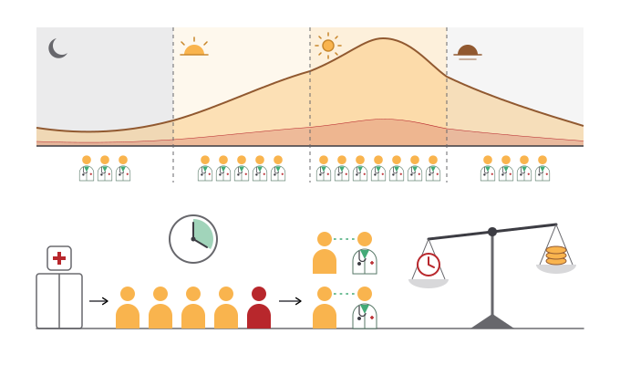
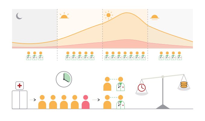
Objective: For each shift, determine the minimum number of doctors such that at least 90% of patients wait no more than 20 minutes.

---

Data

From historical data, the average inter-arrival time $\mu_A$ per shift is known:

Shift	Time	Patients/h	$\mu_A$ (min)
Night	00–06	2	30
Morning	06–12	6	10
Afternoon	12–18	10	6
Evening	18–24	4	15

• Mean treatment duration: $\mu_B = 30$ minutes, independent of time of day
• Exponential distribution is assumed for both inter-arrival and service times

Minimum stability capacity $c_{\min} = \lceil \mu_B / \mu_A \rceil$: Night 2, Morning 4, Afternoon 6, Evening 3. However, stability alone does not guarantee an adequate service level.

---

Step 1: Single-Shift Base Model (Afternoon)

Starting with the peak-load shift (Afternoon, $\mu_A = 6$, $\mu_B = 30$) at minimum capacity $c = 6$:

• Utilization: $\rho = \mu_B / (c \cdot \mu_A) = 30 / (6 \cdot 6) = 83\%$
• The queue exhibits strong fluctuations — typical at high utilization

---

Step 2: Measuring Service Level

A Function block checks per patient whether waiting time ≤ 20 minutes (1 = yes, 0 = no). A Statistics block averages across all patients to obtain the service level.

• 50 replications of 10,000 time units each (plus 500 time units warm-up)
• Result at $c = 6$: service level ≈ 69% ± 2% — well below 90%

---

Step 3: Sweep Over Capacity (Afternoon Shift)

Incrementally increasing capacity $c$ yields:

Capacity $c$	Utilization $\rho$	Service level ($W_q \le 20$ min)
6	83%	≈ 65%
7	71%	≈ 83%
8	63%	≈ 92%
9	56%	≈ 97%

→ At $c = 8$ the target service level of ≥ 90% is first met. Two additional doctors beyond the stability minimum are required.

---

Step 4: Automated Grid Search with Explorer Block

The Explorer block automates parameter variation across all 4 shifts × 10 capacity levels = 40 scenarios:

for (const mu_A of [30, 10, 6, 15]) {
  for (const c of [1, 2, 3, 4, 5, 6, 7, 8, 9, 10]) {
    M[0] = mu_A;  // set inter-arrival time
    M[1] = c;     // set capacity
    yield;        // start simulation run (one edition)
  }
}

Wiring:

• Explorer M[0] → RandomExponential mean ($\mu_A$)
• Explorer M[1] → Perform capacity ($c$)
• Explorer M[0], M[1] → Statistics P[0], P[1] (for logging which shift/capacity)
• Queue wait → Function (0/1 indicator) → Statistics P[2]

Statistics block settings:

• 40 editions (4 shifts × 10 capacities)
• 10 numBatches per edition → confidence interval per edition via batch means
• 500 time units warmupWidth to exclude the transient phase
• Total duration 10,500 time units → each batch covers 1,000 time units

---

Results

Critical Capacity c* (service level ≥ 90%)

Shift	$\mu_A$ (min)	$c^*$
Night ($\mu_A = 30$)	30	3
Evening ($\mu_A = 15$)	15	4
Morning ($\mu_A = 10$)	10	5
Afternoon ($\mu_A = 6$)	6	7

Observations:

• The shorter $\mu_A$ (more patients per hour), the more capacity is required
• Confidence intervals are widest at the critical capacities — estimation is most uncertain exactly where the service level crosses the 90% threshold
• At ≈ 0% or ≈ 100% service level: negligible uncertainty (result is unambiguous)

---

Staffing Plan

The simulation yields the following minimum staffing plan:

Shift	Time	Doctors
Night	00–06	3
Morning	06–12	5
Afternoon	12–18	7
Evening	18–24	4

Total requirement: 3 + 5 + 7 + 4 = 19 doctor-shifts per 24 hours

This plan forms the basis for scheduling. In practice, additional factors apply: breaks, handover times, absences, part-time arrangements, etc.

---

Extended Model: Emergency Priority with Gamma-Distributed Treatment Times

This model extends the base model with:

• Gamma-distributed treatment times (shape $k = 2$, scale $\theta = 25$, giving mean $\mu_B = 50$ min) — more realistic than exponential for medical treatment
• A separate emergency arrival stream ($\mu_N = 180$ min inter-arrival), prioritized via a Select block
• Priority logic: the Select block routes an emergency patient whenever the emergency queue is non-empty (checked via a Function block on queue1.measureLoad); otherwise a regular patient is served

Priority Logic

The Select block routes from input 1 (emergency queue) when its selection parameter $S = 1$, and from input 0 (regular queue) when $S = 0$. The Function block:

M[0] = P[0] > 0 ? 1 : 0

reads the current load of the emergency queue (queue1.measureLoad) and outputs 1 whenever at least one emergency patient is waiting, thus overriding regular patients.

Key Differences from the Base Model

Aspect	Base model	Extended model
Treatment time distribution	Exponential ($\mu = 30$)	Gamma ($k=2$, $\theta=25$, mean=50)
Arrival streams	1 (regular only)	2 (regular + emergency)
Routing	Direct queue → perform	Select block with priority
Regular inter-arrival	configurable	$\mu_A = 15$ min
Emergency inter-arrival	—	$\mu_N = 180$ min
Capacity	configurable	$c = 4$

---

Exercises

Exercise 1: Morning Shift

Parametrize the model for the Morning shift ($\mu_A = 10$, $\mu_B = 30$):

1. Start at minimum capacity $c = 4$.
2. Increase $c$ stepwise until service level ≥ 90%.
3. Document results in a table analogous to the Afternoon analysis.

Exercise 2: Sensitivity Analysis

Using the Afternoon model ($\mu_A = 6$, $\mu_B = 30$), investigate the effect of:

1. A stricter quality target: 95% instead of 90% service level
2. A shorter waiting time threshold: 10 minutes instead of 20 minutes
3. Mean treatment duration increasing to $\mu_B = 45$ minutes

How many additional doctors are needed in each case?

Exercise 3: Two-Stage Process (Triage + Treatment)

Extend the model with an upstream triage stage:

1. Triage (initial assessment): $\mu_B = 5$ min, $c_1 = 1$
2. Treatment: $\mu_C = 30$ min, $c_2$ = to be determined

Tasks:

1. Build two Queue–Perform pairs in series.
2. Determine $c_2$ for the Afternoon shift ($\mu_A = 6$) so that service level ≥ 90%.
3. Measure waiting time before triage and before treatment separately.
4. Compare with the result without triage — where is the bottleneck?

Exercise 4: Emergency Prioritization

Extend the Afternoon model with an emergency entrance using a Select block:

• Regular patients: $\mu_A = 6$ min
• Emergency patients: $\mu_N = 60$ min (less frequent)
• Emergencies are prioritized (Select block with priority logic)

Tasks:

1. Build the model with two Arrive–Queue paths merged via a Select block.
2. Measure service level separately for regular and emergency patients.
3. How does staffing need change compared to the model without emergencies?
4. What happens to regular patient service level as the emergency arrival rate increases?