Quisim Examples

---

Creating Simulation Models from UML State Diagrams

UML State Diagrams — Overview

UML (Unified Modeling Language) is a modeling language for concisely describing a system, widely used in software engineering. A state diagram models the behavior of a system or object in response to events.

A state diagram consists of:

• States — describe the system's current phase or condition; shown as labeled rectangles
• Events — signals or environmental changes that may trigger state transitions
• Transitions — arrows from one state to another, optionally labeled with: the triggering event, a guard condition (must be true for the transition to occur), and an action executed as a result
• Actions — invoked when the system is in a specific state:
  • Entry actions: executed when entering the state
  • Do actions: executed continuously while in the state
  • Exit actions: executed when leaving the state

---

Case Study: Machine State Diagram (Deterministic)

State diagram:

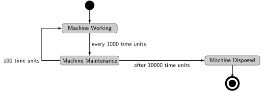
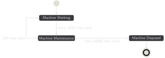
The machine cycles through Working (1000 time units) and Maintenance (100 time units). After accumulating 10,000 total time units, the machine is disposed.

Key modeling idea: The entity carries a time attribute that accumulates the elapsed working and maintenance time. A Function block (check end of life) uses this to decide whether to dispose the entity or loop back to Working.

Quisim model:

Model codeOpen in Quisim

// Quisim licensed for academic use only
Provide { id: provide0; x:16; y:64 }
Meter { id: meter0; x:112; y:64; capacity:1 }
Pipe { from: meter0.outlet; to: set0.inlet }
Queue { id: queue0; x:272; y:160 }
Pipe { from: queue0.outlet; to: perform0.inlet }
Perform { id: perform0; x:368; y:46; capacity:1; label:"Working"; width:48 }
Get { id: get1; x:464; y:64; attribute:"time" }
Wire { from: get1.measureValue; to: function1.parameters[0] }
Pipe { from: get1.outlet; to: set1.inlet }
Pipe { from: perform0.outlet; to: get1.inlet }
Set { id: set1; x:544; y:64; attribute:"time" }
Pipe { from: set1.outlet; to: perform1.inlet }
Perform { id: perform1; x:656; y:46; label:"Maintenance" }
Pipe { from: perform1.outlet; to: get0.inlet }
Pipe { from: provide0.outlet; to: meter0.inlet }
Get { id: get0; x:752; y:64; attribute:"time" }
Pipe { from: get0.outlet; to: set2.inlet }
Wire { from: get0.measureValue; to: report0.parameters[0]; bend:60 }
Report { id: report0; x:592; y:304; height:87 }
Set { id: set0; x:192; y:64; attribute:"time"; value:0 }
Pipe { from: set0.outlet; to: queue0.inlet }
Decide { id: decide0; x:992; y:160; label:"End of life?" }
Pipe { from: decide0.outlets[0]; to: queue0.inlet; bend:-57 }
Leave { id: leave0; x:1088; y:174; label:"Dispose" }
Pipe { from: decide0.outlets[1]; to: leave0.inlet }
Function { id: function0; x:816; y:304; numParameters:1; code:"M[0]=P[0]<10000?0:1"; label:"check end of life"; height:48 }
Wire { from: function0.measures[0]; to: decide0.parameters[0] }
Function { id: function1; x:432; y:208; numParameters:2; label:"add time delta"; code:"M[0] = P[0]+P[1]" }
Wire { from: function1.measures[0]; to: function0.parameters[0] }
Wire { from: function1.measures[0]; to: set1.parameterValue }
Number { id: number0; label:"work time"; value:1000; x:288; y:304 }
Wire { from: number0.measureValue; to: function1.parameters[1] }
Wire { from: number0.measureValue; to: perform0.parameterDuration }
Steering { id: steering0; duration:20000; x:16; y:192 }
Number { id: number1; x:432; y:304; value:100; label:"maintenance time"; width:137 }
Wire { from: number1.measureValue; to: perform1.parameterDuration }
Set { id: set2; x:848; y:64; attribute:"time" }
Pipe { from: set2.outlet; to: decide0.inlet }
Wire { from: get0.measureValue; to: function2.parameters[0] }
Wire { from: number1.measureValue; to: function2.parameters[1] }
Function { id: function2; x:640; y:208; label:"add maintenance time"; width:160; numParameters:2; code:"M[0]=P[0]+P[1]" }
Wire { from: function2.measures[0]; to: set2.parameterValue }

---

Case Study: Machine State Diagram (Probabilistic Disposal)

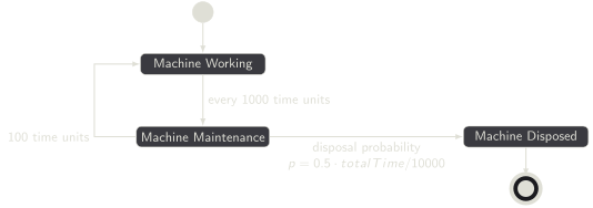
Extension: Instead of a fixed disposal time of 10,000 time units, the machine is disposed of with a probability that grows over time:

$$p = 0.5 \cdot \text{totalTime} / 10000$$

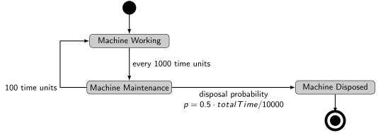
Deciding disposal with a Uniform distribution:

To use the Decide block with probability $p$, a Uniform distribution on interval $[a, b]$ is used such that $P[U \ge 1] = p$. This is achieved by setting:

$$a = p, \quad b = 1 + p$$

The Function block labeled check end of life computes both bounds from the accumulated totalTime:

let prob = 0.5 * P[0] / 10000
M = [prob, 1 + prob]

The two outputs drive the lower and upper sockets of a RandomUniform block, whose output goes to the Decide block's selection parameter.

Quisim model:

Model codeOpen in Quisim

// Quisim licensed for academic use only
Provide { id: provide0; x:16; y:64 }
Meter { id: meter0; x:112; y:64; capacity:1 }
Pipe { from: meter0.outlet; to: set0.inlet }
Queue { id: queue0; x:272; y:160 }
Pipe { from: queue0.outlet; to: perform0.inlet }
Perform { id: perform0; x:368; y:46; capacity:1; label:"Working"; width:48 }
Get { id: get1; x:464; y:64; attribute:"time" }
Wire { from: get1.measureValue; to: function1.parameters[0] }
Pipe { from: get1.outlet; to: set1.inlet }
Pipe { from: perform0.outlet; to: get1.inlet }
Set { id: set1; x:544; y:64; attribute:"time" }
Pipe { from: set1.outlet; to: perform1.inlet }
Perform { id: perform1; x:656; y:46; label:"Maintenance" }
Pipe { from: perform1.outlet; to: get0.inlet }
Pipe { from: provide0.outlet; to: meter0.inlet }
Get { id: get0; x:752; y:64; attribute:"time" }
Pipe { from: get0.outlet; to: set2.inlet }
Wire { from: get0.measureValue; to: report0.parameters[0]; bend:60 }
Report { id: report0; x:592; y:304; height:87 }
Set { id: set0; x:192; y:64; attribute:"time"; value:0 }
Pipe { from: set0.outlet; to: queue0.inlet }
Decide { id: decide0; x:992; y:160; label:"End of life?" }
Pipe { from: decide0.outlets[0]; to: queue0.inlet; bend:-57 }
Leave { id: leave0; x:1088; y:174; label:"Dispose" }
Pipe { from: decide0.outlets[1]; to: leave0.inlet }
Function { id: function1; x:432; y:208; numParameters:2; label:"add time delta"; code:"M[0] = P[0]+P[1]" }
Wire { from: function1.measures[0]; to: set1.parameterValue }
Number { id: number0; label:"work time"; value:1000; x:288; y:304 }
Wire { from: number0.measureValue; to: function1.parameters[1] }
Wire { from: number0.measureValue; to: perform0.parameterDuration }
Steering { id: steering0; duration:20000; x:16; y:192 }
Number { id: number1; x:432; y:304; value:100; label:"maintenance time"; width:137 }
Wire { from: number1.measureValue; to: perform1.parameterDuration }
Set { id: set2; x:848; y:64; attribute:"time" }
Pipe { from: set2.outlet; to: decide0.inlet }
Wire { from: get0.measureValue; to: function2.parameters[0] }
Wire { from: number1.measureValue; to: function2.parameters[1] }
Function { id: function2; x:640; y:208; label:"add maintenance time"; width:160; numParameters:2; code:"M[0]=P[0]+P[1]" }
Wire { from: function2.measures[0]; to: set2.parameterValue }
RandomUniform { id: randomuniform0; x:884; y:160; fillColor:"#f0aca1" }
Wire { from: randomuniform0.measureRandomVariate; to: decide0.parameters[0] }
Wire { from: function2.measures[0]; to: function4.parameters[0] }
Function { id: function4; x:884; y:304; numParameters:1; code:"let prob=0.5*P[0]/10000\nM=[prob, 1+prob]"; label:"check end of life"; fillColor:"#f0aca1"; numMeasures:2 }
Wire { from: function4.measures[1]; to: randomuniform0.parameterUpper }
Wire { from: function4.measures[0]; to: randomuniform0.parameterLower }

---

Virus Spread

State Diagram

The virus spread model tracks individuals through five states:

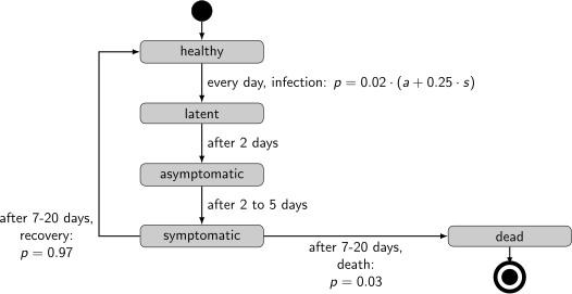
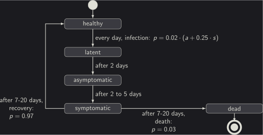
Where $a$ = number of asymptomatic persons and $s$ = number of symptomatic persons currently in the system.

Model Construction

The simulation starts with 39 people in the healthy state and 1 immediately injected into the latent state.

Healthy state: modeled by a Perform block with infinite capacity and duration 1 time unit, which drives one person at a time through a infection? Decide block.

Infection probability: p = 0.02·(a + 0.25·s), implemented in a Function block:

M[1] = Math.min(2, 1 + 0.02*(P[0] + 0.25*P[1]));
M[0] = M[1] - 1

The two outputs set the lower and upper of a RandomUniform block feeding the infection? Decide block.

Disease progression after infection:

• Latent: constant 2 time units
• Asymptomatic: Uniform [2, 5]
• Symptomatic: Uniform [7, 20]

Death probability: 3%, modeled with a Uniform distribution on [0.03, 1.03].

Outcome: either recovery (return to healthy queue) or death (Leave block).

Quisim model:

Model codeOpen in Quisim

Steering { id: steering0; x:33; y:491; duration:100; height:48 }
Perform { id: queue0; x:300; y:94; label:"healthy"; duration:1; capacity:Infinity }
Pipe { from: queue0.outlet; to: decide0.inlet }
Wire { from: queue0.measureLoad; to: chart0.parameters[0] }
Perform { id: perform0; x:543; y:108; duration:2; label:"latent"; capacity:Infinity }
Pipe { from: perform0.outlet; to: perform2.inlet }
Decide { id: decide0; x:415; y:112; label:"infection?" }
Pipe { from: decide0.outlets[1]; to: perform0.inlet }
Pipe { from: decide0.outlets[0]; to: queue0.inlet; bend:-50 }
Perform { id: perform2; x:642; y:108; label:"asymptomatic"; capacity:Infinity }
Pipe { from: perform2.outlet; to: perform3.inlet }
Perform { id: perform3; x:745; y:108; label:"symptomatic"; capacity:Infinity }
Wire { from: perform3.measureLoad; to: function0.parameters[1] }
Wire { from: perform3.measureLoad; to: chart0.parameters[1] }
Decide { id: decide1; x:844; y:126; label:"death?" }
Pipe { from: decide1.outlets[0]; to: queue0.inlet; bend:-150 }
Leave { id: leave0; label:"dead"; x:945; y:140 }
Pipe { from: decide1.outlets[1]; to: leave0.inlet }
Pipe { from: perform3.outlet; to: decide1.inlet }
Provide { id: provide0; x:35; y:35 }
Pipe { from: provide0.outlet; to: meter1.inlet }
Pipe { from: provide0.outlet; to: meter0.inlet }
Meter { id: meter0; x:112; y:112; capacity:39 }
Pipe { from: meter0.outlet; to: queue0.inlet }
RandomUniform { id: randomuniform0; x:311; y:191 }
Wire { from: randomuniform0.measureRandomVariate; to: decide0.parameters[0] }
Wire { from: perform2.measureLoad; to: function0.parameters[0] }
Function { id: function0; x:36; y:197; numParameters:2; code:"M[1]=Math.min(2,1+.02*(P[0]+0.25*P[1]));\nM[0]=M[1]-1"; numMeasures:2 }
Wire { from: function0.measures[1]; to: randomuniform0.parameterUpper; bend:0 }
Wire { from: function0.measures[0]; to: randomuniform0.parameterLower; bend:0 }
Meter { id: meter1; x:200; y:42; capacity:1 }
Pipe { from: meter1.outlet; to: perform0.inlet; bend:-30 }
Wire { from: leave0.measureNumPassed; to: chart0.parameters[2] }
Chart { id: chart0; x:35; y:311; numParameters:3; height:119; width:956; fillColor:"#999999" }
RandomUniform { id: randomuniform2; x:536; y:196; lower:2; upper:5 }
Wire { from: randomuniform2.measureRandomVariate; to: perform2.parameterDuration }
RandomUniform { id: randomuniform3; x:651; y:196; lower:7; upper:20 }
Wire { from: randomuniform3.measureRandomVariate; to: perform3.parameterDuration }
RandomUniform { id: randomuniform5; x:765; y:196; upper:1.03; lower:0.03 }
Wire { from: randomuniform5.measureRandomVariate; to: decide1.parameters[0] }

---

Production Simulation

Workflow Types

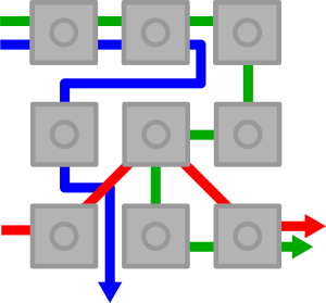
Three fundamental production workflow forms:

• Parallel Resources — orders are distributed across multiple resources working in parallel

  

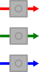
• Flow Shop — orders pass through multiple resources sequentially in the same order for every job

  

• Job Shop — orders pass through multiple resources sequentially, but the order is specific to each job

  

---

Flow Shop Production

Setup:

• Two sequential machines
• Exactly one buffer space before the second machine
• 20 orders, all available at the start
• Processing times: Uniform[200, 600] on machine 1; Uniform[100, 400] on machine 2
• KPI: completion time of the last order (read from the LT output of a Meter block)

Quisim model:

The Provide and Meter (capacity 20) pair releases the 20 orders at time 0. The Statistics block uses quantile: 1, so it reports the largest LT per run, which is the completion time of the last order. A Function block sets the number of replications from the edition number EN: R = 100 + EN · 100.

Model codeOpen in Quisim

RandomUniform { id: randomuniform0; lower:200; upper:600; seed:2000 }
Wire { from: randomuniform0.measureRandomVariate; to: perform0.parameterDuration }
RandomUniform { id: randomuniform1; lower:100; upper:400; seed:1000 }
Wire { from: randomuniform1.measureRandomVariate; to: perform1.parameterDuration }
Provide { id: provide0 }
Pipe { from: provide0.outlet; to: meter0.inlet }
Meter { id: meter0; capacity:20 }
Pipe { from: meter0.outlet; to: queue0.inlet }
Queue { id: queue0 }
Pipe { from: queue0.outlet; to: perform0.inlet }
Perform { id: perform0 }
Pipe { from: perform0.outlet; to: queue1.inlet }
Queue { id: queue1; capacity:1 }
Pipe { from: queue1.outlet; to: perform1.inlet }
Perform { id: perform1 }
Pipe { from: perform1.outlet; to: meter1.inlet }
Meter { id: meter1 }
Pipe { from: meter1.outlet; to: leave0.inlet }
Leave { id: leave0 }
Steering { id: steering0; editions:10 }
Statistics { id: statistics0; quantile: 1 }
Wire { from: meter1.measureLastTime; to: statistics0.parameters[0] }
Wire { from: steering0.measureEdition; to: function0.parameters[0] }
Function { id: function0; code:"M[0]=100+P[0]*100" }
Wire { from: function0.measures[0]; to: steering0.parameterReplications }

Confidence Interval vs. Number of Replications

Running the flow shop model with an increasing number of replications (100 to 5000), the 95% confidence radius shrinks approximately as:

$$\text{confidence radius} \approx \frac{1000}{\sqrt{R}}$$

Replications	Average	95% Radius
100	8274.48	104.65
200	8256.81	66.64
300	8284.65	55.79
400	8293.93	49.92
500	8294.81	44.99
1000	8283.57	31.47
2000	—	~22.77
5000	—	~14.23

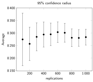
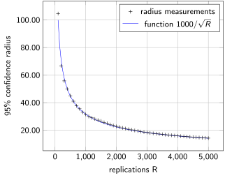
The confidence interval (radius) shrinks at a rate of order $1/\sqrt{R}$.

---

Flow Shop Production with Re-Work

Extension: 10% of completed jobs fail quality control and must pass through both machines again.

Since seeds are set, a system comparison (with vs. without re-work) using CRN is straightforward. Comparing means using a Python t-test on the difference $D = A - B$ across replications shows that none of the 95% confidence intervals for the difference contain zero — the system without defects is significantly better.

Quisim model:

After machine 2, a Decide block checks quality. A RandomUniform on [0.1, 1.1] sends 10% of the jobs (values ≥ 1) back to the queue before machine 1. The simulation length is raised to 20,000 so that all re-worked jobs can finish.

Model codeOpen in Quisim

Steering { id: steering0; editions:1; duration:20000 }
RandomUniform { id: randomuniform0; lower:200; upper:600; seed:2000 }
Wire { from: randomuniform0.measureRandomVariate; to: perform0.parameterDuration }
RandomUniform { id: randomuniform1; lower:100; upper:400; seed:1000 }
Wire { from: randomuniform1.measureRandomVariate; to: perform1.parameterDuration }
Provide { id: provide0 }
Pipe { from: provide0.outlet; to: meter0.inlet }
Meter { id: meter0; capacity:20 }
Pipe { from: meter0.outlet; to: queue0.inlet }
Queue { id: queue0 }
Pipe { from: queue0.outlet; to: perform0.inlet }
Perform { id: perform0 }
Pipe { from: perform0.outlet; to: queue1.inlet }
Queue { id: queue1; capacity:1 }
Pipe { from: queue1.outlet; to: perform1.inlet }
Perform { id: perform1 }
RandomUniform { id: randomuniform2; lower:0.1; upper:1.1 }
Wire { from: randomuniform2.measureRandomVariate; to: decide0.parameters[0] }
Decide { id: decide0; label:"defect?" }
Pipe { from: decide0.outlets[1]; to: queue0.inlet; bend:50 }
Pipe { from: decide0.outlets[0]; to: meter1.inlet }
Pipe { from: perform1.outlet; to: decide0.inlet }
Meter { id: meter1 }
Number { id: number0 }
Wire { from: meter1.measureLastTime; to: number0.parameterValue }
Pipe { from: meter1.outlet; to: leave0.inlet }
Leave { id: leave0 }

---

Flow Shop with Recycling

Extension of re-work: Instead of always re-running both machines, a separate testing step (exponentially distributed, mean 200 time units) allows 50% of defective jobs to skip the first machine.

Analysis over 20×20 runs shows that only 6 of 20 confidence intervals for the difference are above zero, meaning it is not statistically clear whether this recycling step improves performance.

Quisim model:

Defective jobs go to a testing step (Perform with infinite capacity, Exponential with mean 200). A second Decide block, driven by a RandomUniform on [0, 2], then sends each tested job back either to machine 1 or straight to the queue before machine 2, each with probability 50%.

Model codeOpen in Quisim

Steering { id: steering0; duration:20000; replications:400 }
RandomUniform { id: randomuniform0; lower:200; upper:600; seed:2000 }
Wire { from: randomuniform0.measureRandomVariate; to: perform0.parameterDuration }
RandomUniform { id: randomuniform1; lower:100; upper:400; seed:1000 }
Wire { from: randomuniform1.measureRandomVariate; to: perform1.parameterDuration }
Provide { id: provide0 }
Pipe { from: provide0.outlet; to: meter0.inlet }
Meter { id: meter0; capacity:20 }
Pipe { from: meter0.outlet; to: queue0.inlet }
Queue { id: queue0 }
Pipe { from: queue0.outlet; to: perform0.inlet }
Perform { id: perform0 }
Pipe { from: perform0.outlet; to: queue1.inlet }
Queue { id: queue1; capacity:1 }
Pipe { from: queue1.outlet; to: perform1.inlet }
Perform { id: perform1 }
RandomUniform { id: randomuniform2; lower:0.1; upper:1.1 }
Wire { from: randomuniform2.measureRandomVariate; to: decide0.parameters[0] }
Decide { id: decide0; label:"defect?" }
RandomExponential { id: randomexponential0; mean:200 }
Wire { from: randomexponential0.measureRandomVariate; to: perform2.parameterDuration }
Perform { id: perform2; capacity:Infinity; label:"testing" }
RandomUniform { id: randomuniform3; upper:2 }
Wire { from: randomuniform3.measureRandomVariate; to: decide1.parameters[0] }
Decide { id: decide1; label:"skip machine 1?" }
Pipe { from: decide1.outlets[1]; to: queue1.inlet; bend:-100 }
Pipe { from: decide1.outlets[0]; to: queue0.inlet; bend:-100 }
Pipe { from: perform2.outlet; to: decide1.inlet }
Pipe { from: decide0.outlets[1]; to: perform2.inlet }
Pipe { from: decide0.outlets[0]; to: meter1.inlet }
Pipe { from: perform1.outlet; to: decide0.inlet }
Meter { id: meter1 }
Number { id: number0 }
Wire { from: meter1.measureLastTime; to: number0.parameterValue }
Pipe { from: meter1.outlet; to: leave0.inlet }
Leave { id: leave0 }

---

Design of Experiments (DoE)

The 2^k Factorial Design

When comparing multiple system configurations, a $2^k$ factorial design systematically tests all combinations of $k$ factors, each at two levels (−1 and +1), giving $2^k$ experiments total.

Example factors (a flow shop with two machines and exponential processing times):

• Factor A: mean processing time on machine 1 is 350 (+1) or 400 (−1)
• Factor B: mean processing time on machine 2 is 250 (+1) or 300 (−1)

The result $\mathcal{L}$ is the average completion time of the last of 20 orders (100 replications):

Experiment	Factor A	Factor B	Result $\mathcal{L}$
1	−1	−1	8547
2	+1	−1	8068
3	−1	+1	8322
4	+1	+1	7686

Contrast Method — Main Effects

The effect $E_Z$ of parameter $Z$ is the average change in performance $\mathcal{L}$ when $Z$ moves from its low (−1) to high (+1) level:

$$E_Z = \frac{1}{|Z_{+1}|}\sum_{v \in Z_{+1}} \mathcal{L}_v - \frac{1}{|Z_{-1}|}\sum_{v \in Z_{-1}} \mathcal{L}_v$$

For the example above:

$$E_A = \frac{1}{2}(8068 + 7686) - \frac{1}{2}(8547 + 8322) = -557.5$$

$$E_B = \frac{1}{2}(8322 + 7686) - \frac{1}{2}(8547 + 8068) = -303.5$$

Contrast Method — Interaction Effect

The interaction effect $E_{ZX}$ between factors $Z$ and $X$ is computed by assigning +1 when both factors are at the same level and −1 otherwise (multiply signs):

Experiment	A	B	$A \cdot B$	$\mathcal{L}$
1	−1	−1	+1	8547
2	+1	−1	−1	8068
3	−1	+1	−1	8322
4	+1	+1	+1	7686

$$E_{AB} = \frac{1}{2}(8547 + 7686) - \frac{1}{2}(8068 + 8322) = -78.5$$

The interaction is small compared to the main effects: speeding up one machine helps only slightly more when the other machine is sped up as well.

For three or more factors, higher-order interactions (ABC, etc.) are computed by multiplying the corresponding sign columns.

Implementing DoE in Quisim

Use a Function block to convert the edition number EN into a binary configuration. For a $2^k$ design with $k=2$, we need $2^2 = 4$ editions:

let k = 2;
let F = ((1 << k) + P[0]).toString(2)  // binary string, e.g. "110"
// Check individual bits:
F[1] == 1   // Factor A active?
F[2] == 1   // Factor B active?

Results are read from the Statistics block, one row per edition.

Quisim model:

Factor A lowers the mean on machine 1 from 400 to 350. Factor B lowers the mean on machine 2 from 300 to 250. Edition EN = 0…3 selects the configuration. As in the Flow Shop model, the Statistics block uses quantile: 1, so it reports the largest LT per run, which is the completion time of the last order. The random blocks are seeded, so every run reproduces the table above, and all four configurations use common random numbers.

Model codeOpen in Quisim

Steering { id: steering0; editions:4; replications:100 }
Function { id: function0; numMeasures:2; code:"let k=2\nlet F=((1<<k)+P[0]).toString(2)\nM[0]=F[1]==1?350:400\nM[1]=F[2]==1?250:300" }
Wire { from: steering0.measureEdition; to: function0.parameters[0] }
Wire { from: function0.measures[0]; to: rnd0.parameterMean }
Wire { from: function0.measures[1]; to: rnd1.parameterMean; bend:50 }
RandomExponential { id: rnd0; seed:2000 }
Wire { from: rnd0.measureRandomVariate; to: perform0.parameterDuration }
RandomExponential { id: rnd1; seed:1000 }
Wire { from: rnd1.measureRandomVariate; to: perform1.parameterDuration }
Provide { id: provide0 }
Pipe { from: provide0.outlet; to: meter0.inlet }
Meter { id: meter0; capacity:20 }
Pipe { from: meter0.outlet; to: queue0.inlet }
Queue { id: queue0 }
Pipe { from: queue0.outlet; to: perform0.inlet }
Perform { id: perform0 }
Pipe { from: perform0.outlet; to: queue1.inlet }
Queue { id: queue1 }
Pipe { from: queue1.outlet; to: perform1.inlet }
Perform { id: perform1 }
Pipe { from: perform1.outlet; to: meter1.inlet }
Meter { id: meter1 }
Statistics { id: statistics0; quantile: 1 }
Wire { from: meter1.measureLastTime; to: statistics0.parameters[0] }
Pipe { from: meter1.outlet; to: leave0.inlet }
Leave { id: leave0 }

---

Simulation Optimization

Overview

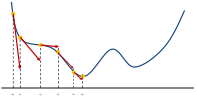
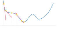
Simulation optimization finds the best input parameters for a simulation-based system. Challenges include noisy simulation outputs (stochastic effects) and high computational cost. Common methods:

• Grid search — evaluates a discrete set of parameter values
• Stochastic Approximation — e.g., the Kiefer-Wolfowitz algorithm for noisy environments
• Metaheuristics — genetic algorithms, simulated annealing

---

Grid Search Example: M/M/10 Queue

Problem: Given an M/M/10 queue with mean service time $1/\mu = 100$, find mean inter-arrival time $1/\lambda$ to minimize total cost:

$$\mathcal{L}(1/\lambda) = \hat{L} + 1/\lambda$$

where $\hat{L}$ is the time-average queue length from simulation.

Quisim model:

Each edition EN tests one grid point, $1/\lambda = EN + 1$. The Statistics block averages the queue length over time.

Model codeOpen in Quisim

Steering { id: steering0; duration:10000; editions:20; replications:20 }
Wire { from: steering0.measureEdition; to: function0.parameters[0] }
Function { id: function0; code:"M[0]=P[0]+1"; label:"1/λ" }
Wire { from: function0.measures[0]; to: rnd0.parameterMean }
RandomExponential { id:rnd0; seed:88 }
RandomExponential { id:rnd1; mean:100; seed:143 }
Wire { from:rnd0.measureRandomVariate; to:arrive0.parameterDuration }
Wire { from:rnd1.measureRandomVariate; to:perform0.parameterDuration }
Arrive { id:arrive0 }
Pipe { from:arrive0.outlet; to:queue0.inlet }
Queue { id:queue0 }
Pipe { from:queue0.outlet; to:perform0.inlet }
Perform { id:perform0; capacity:10 }
Pipe { from:perform0.outlet; to:leave0.inlet }
Leave { id:leave0 }
Wire { from: queue0.measureLoad; to: statistics0.parameters[0] }
Statistics { id: statistics0; timeAverage:true; label:"queue length" }

Grid search over $1/\lambda = 1, 2, \ldots, 20$ (simulation length 10,000, 20 replications) yields:

$1/\lambda$	$\hat{L}$	$\mathcal{L}$
10	19.43	29.43
11	5.27	16.27
12	1.99	13.99
13	1.00	14.00
14	0.54	14.54

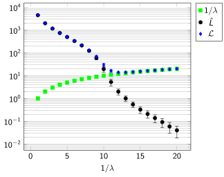
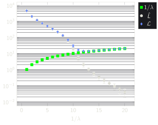
The minimum is near $1/\lambda \approx 12$–$12.5$. A refined search over [12.0, 13.9] in steps of 0.1 shows the minimum near 12.4–12.5, but confidence intervals overlap — CRN is needed for a definitive comparison.

$1/\lambda$	$\hat{L}$	95% conf. radius	$\mathcal{L}$
12.0	1.99	0.59	13.99
12.1	1.84	0.54	13.94
12.2	1.71	0.49	13.91
12.3	1.58	0.44	13.88
12.4	1.47	0.40	13.87
12.5	1.37	0.38	13.87
12.6	1.28	0.35	13.88
12.7	1.21	0.33	13.91
12.8	1.14	0.31	13.94
12.9	1.07	0.29	13.97
13.0	1.00	0.27	14.00
13.1	0.94	0.26	14.04
13.2	0.88	0.24	14.08
13.3	0.83	0.23	14.13
13.4	0.78	0.21	14.18
13.5	0.73	0.20	14.23
13.6	0.68	0.19	14.28
13.7	0.64	0.18	14.34
13.8	0.61	0.17	14.41
13.9	0.57	0.16	14.47

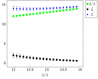
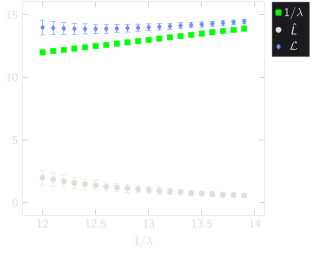
Note on overlapping confidence intervals: Even with CRN, the 95% confidence intervals for adjacent parameter values near the optimum overlap, so no single value can be unambiguously declared best. This motivates the use of dedicated optimization algorithms.

Comparing neighbouring grid points over 20 replications with common random numbers, $\mathcal{D}$ is the difference per replication:

$\mathcal{L}(12.4)$	$\mathcal{L}(12.5)$	$\mathcal{D}$		$\mathcal{L}(12.5)$	$\mathcal{L}(12.6)$	$\mathcal{D}$
13.710	13.729	−0.019		13.729	13.755	−0.026
13.245	13.283	−0.038		13.283	13.317	−0.034
13.784	13.783	0.001		13.783	13.788	−0.005
13.820	13.831	−0.010		13.831	13.848	−0.017
14.713	14.691	0.023		14.691	14.675	0.016
13.280	13.295	−0.015		13.295	13.286	0.009
12.767	12.793	−0.026		12.793	12.876	−0.083
13.198	13.253	−0.055		13.253	13.309	−0.056
14.994	14.932	0.062		14.932	14.894	0.038
14.735	14.721	0.014		14.721	14.711	0.009
14.441	14.419	0.022		14.419	14.397	0.021
14.392	14.390	0.002		14.390	14.391	−0.002
17.420	17.000	0.420		17.000	16.640	0.360
13.596	13.602	−0.006		13.602	13.621	−0.018
13.388	13.419	−0.031		13.419	13.460	−0.041
14.542	14.555	−0.013		14.555	14.558	−0.003
14.265	14.241	0.024		14.241	14.238	0.003
12.956	13.015	−0.059		13.015	13.079	−0.063
15.149	14.968	0.181		14.968	14.845	0.123
13.770	13.765	0.005		13.765	13.756	0.009
	$\bar{\mathcal{D}}$	0.024			$\bar{\mathcal{D}}$	0.012
	95% CI	[−0.027, 0.075]			95% CI	[−0.033, 0.056]

Both confidence intervals for the difference contain zero.

---

Kiefer-Wolfowitz Algorithm (FDSA)

Also called Finite Difference Stochastic Approximation. Iteratively estimates the gradient using finite differences and updates the parameter with a decreasing step size.

Parameters:

• Step size: $a_i = a / (i+1)$
• Perturbation size: $c_i = c / \sqrt[3]{i+1}$

Required conditions: $a_i \to 0$, $\sum a_i = \infty$, $c_i \to 0$, $\sum a_i^2/c_i^2 < \infty$

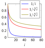
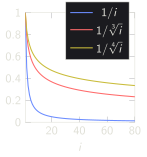
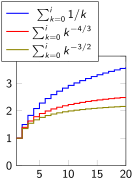
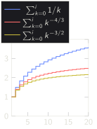
Convergence rate: $O(1/\sqrt[3]{i})$ without CRN; $O(1/\sqrt{i})$ with CRN.

Algorithm:

1. Initialize with $z_1$, set $i \gets 1$
2. Simulate to evaluate $\mathcal{L}(z_i + c_i)$ and $\mathcal{L}(z_i - c_i)$
3. Estimate gradient: $\hat{g}_i = \frac{\mathcal{L}(z_i + c_i) - \mathcal{L}(z_i - c_i)}{2c_i}$
4. Update: $z_{i+1} = z_i - a_i \hat{g}_i$
5. Increment $i$ and repeat until convergence

---

Kiefer-Wolfowitz via Function Block

The Function block stores the iteration state in two JavaScript arrays:

• Z[i] — the parameter value at iteration $i$
• L[2i] = $\mathcal{L}(z_i - c_i)$, L[2i+1] = $\mathcal{L}(z_i + c_i)$

Each iteration requires two editions (one for each perturbed evaluation). The edition number encodes both the iteration index and whether the current run is the + or − perturbation.

Context code (property context):

let a = 1, c = 1
let ai = (i) => a / (i + 1)
let ci = (i) => c / Math.pow(i + 1, 1/3)
let Zinit = 10, numIter = 1000
let Z = Array(numIter), L = Array(2 * numIter)

Init code (property init):

Z[0] = Zinit

Main code (property code):

let i = Math.floor(P[1] / 2)  // iteration = edition / 2 (rounded down)
if (i > 0) Z[i] = Z[i-1] - ai(i-1) * (L[2*i-1] - L[2*i-2]) / (2 * ci(i-1))
M[0] = Z[i]                                       // current guess
M[1] = (P[1] % 2 == 1) ? (Z[i] + ci(i)) : (Z[i] - ci(i))  // parameter value
if (P[0]) L[P[1]] = M[1] + P[2]                  // save result (including 1/λ cost)
M[2] = M[1] + P[2]                               // current cost (for display)

Connect: isFinished F → P[0], edition number E → P[1], queue length L → P[2]. Output M[0] to a Report block (current $z_i$), M[1] to the mean inter arrival time input µ.

Quisim model:

Model codeOpen in Quisim

Steering { id: steering0; duration:10000; editions:20; x:23; y:168 }
Wire { from: steering0.measureEdition; to: function0.parameters[1] }
Wire { from: steering0.measureFinished; to: function0.parameters[0] }
Function { id: function0; numParameters:3; context:"let a=2, c=.1\nlet ai = (i)=>a/(i+1)\nlet ci = (i)=>c/Math.pow(i+1,1/3)\nlet Zinit=12, numIter=1000\nlet Z=Array(numIter), L=Array(2*numIter)"; init:"\nZ[0]=Zinit"; code:"\nlet i = Math.floor(P[1]/2) //iteration number = edition/2 rounded down\nif(i>0) Z[i] = Z[i-1]-ai(i-1)*(L[2*i-1]-L[2*i-2])/(2*ci(i-1)) //iterate\nM[0] = Z[i] // current guess\nM[1] = (P[1]%2==1) ? (Z[i]+ci(i)) : (Z[i]-ci(i)) //set parameter value\nif(P[0]) L[P[1]] = M[1]+P[2] //save result\nM[2] = M[1]+P[2] // current costs"; numMeasures:3; y:11; height:225; width:390; x:168 }
Number { id: number0; x:622; y:169; label:"zᵢ" }
Wire { from: function0.measures[0]; to: number0.parameterValue }
Statistics { id: statistics2; x:20; y:290; label:"1/λ" }
Wire { from: function0.measures[1]; to: statistics2.parameters[0]; bend:35; incline:114; debend:52; decline:204 }
Statistics { id: statistics1; x:254; y:290; label:"costs" }
Wire { from: function0.measures[2]; to: statistics1.parameters[0]; bend:25; incline:59; debend:27; decline:123 }
Wire { from: function0.measures[1]; to: rnd0.parameterMean; bend:30; incline:145; debend:-13; decline:241 }
RandomExponential { id:rnd0; seed:88; y:557; x:86 }
RandomExponential { id:rnd1; mean:100; seed:143; x:394; y:556 }
Wire { from:rnd0.measureRandomVariate; to:arrive0.parameterDuration }
Wire { from:rnd1.measureRandomVariate; to:perform0.parameterDuration }
Arrive { id:arrive0; x:187; y:560 }
Pipe { from:arrive0.outlet; to:queue0.inlet }
Queue { id:queue0; x:293; y:560 }
Pipe { from:queue0.outlet; to:perform0.inlet }
Perform { id:perform0; capacity:10; x:507; y:554 }
Pipe { from:perform0.outlet; to:leave0.inlet }
Leave { id:leave0; x:603; y:572 }
Wire { from: queue0.measureLoad; to: statistics0.parameters[0]; bend:12; incline:-15; debend:4; decline:-10 }
Statistics { id: statistics0; x:484; y:290; timeAverage:true; label:"queue length" }
Wire { from: statistics0.measures[0]; to: function0.parameters[2] }

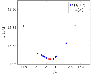
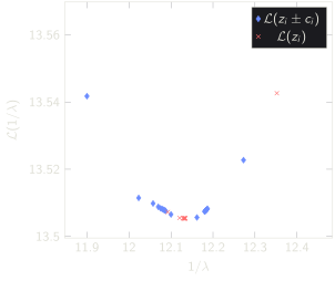
Convergence results (starting from $z_0 = 12$, $a = 2$, $c = 0.1$):

$i$	$z_i$	$\mathcal{L}(z_i)$
1	12.352	13.543
2	12.093	13.507
3	12.120	13.506
4	12.128	13.505
5	12.130	13.505
10	12.134	13.505

---

Explorer Block

The Explorer block is better suited than the Function block for implementing optimization algorithms in Quisim. It loops over multiple simulation runs, using each run's result to configure the next run. A run is started with the yield command.

Data sockets:

• Input sockets M[0], M[1], … : inputs (receive results from simulation)
• Output sockets P[0], P[1], … : outputs (send parameters to simulation)

Kiefer-Wolfowitz via Explorer Block

let a = 1, c = 1;
let ai = (i) => a / (i + 1);
let ci = (i) => c / Math.pow(i + 1, 1/3);
let z = 10;
let i = 0, numIter = 1000;
while (i < numIter) {
    M[0] = z;
    M[1] = z - ci(i); yield; let f_minus = M[2] = P[0];
    M[1] = z + ci(i); yield; let f_plus = M[2] = P[0];
    z = z - ai(i) * (f_plus - f_minus) / (2 * ci(i));
    i = i + 1;
}
M[0] = M[1] = z; yield; M[2] = P[0];

Total number of editions required: 2 * numIter + 1 (two per iteration, one final).

Connect M[0] (current $z_i$) and M[1] (parameter $z_i \pm c_i$) each to a Report block.

Quisim model:

Model codeOpen in Quisim

Steering { id: steering0; duration:10000; editions:20; x:468; y:43 }
Explorer { id: function0; initCode:"let a=2, c=.1\nlet ai = (i)=>a/(i+1)\nlet ci = (i)=>c/Math.pow(i+1,1/3)\nlet Zinit=12, numIter=1000\nlet Z=Array(numIter), L=Array(2*numIter)\nZ[0]=Zinit"; code:"let a = 2, c = 0.1;\nlet ai = (i)=>a/i; let ci = (i)=>c/Math.pow(i,1/3);\nlet z = 12, i = 1, numIter = 1000;\nwhile (i <= numIter) {\n    M[0] = z;\n    M[1] = z - ci(i); yield; let f_minus = M[2] = P[0];\n    M[1] = z + ci(i); yield; let f_plus = M[2] = P[0];\n    z = z - ai(i) * (f_plus - f_minus) / (2 * ci(i));\n    i = i + 1;\n}\nM[0] = M[1] = z; yield; M[2] = P[0];"; numMeasures:3; y:24; x:22; height:181 }
Number { id: number0; x:374; y:163; label:"zᵢ" }
Wire { from: function0.measures[0]; to: number0.parameterValue }
Report { id: statistics2; x:19; y:266; label:"1/λ" }
Wire { from: function0.measures[1]; to: statistics2.parameters[0] }
Report { id: statistics1; x:253; y:266; label:"costs" }
Wire { from: function0.measures[2]; to: statistics1.parameters[0] }
Wire { from: function0.measures[1]; to: rnd0.parameterMean }
RandomExponential { id:rnd0; seed:88; y:529; x:59 }
RandomExponential { id:rnd1; mean:100; seed:143; x:372; y:518 }
Wire { from:rnd0.measureRandomVariate; to:arrive0.parameterDuration }
Wire { from:rnd1.measureRandomVariate; to:perform0.parameterDuration }
Arrive { id:arrive0; x:157; y:532 }
Pipe { from:arrive0.outlet; to:queue0.inlet }
Queue { id:queue0; x:253; y:532 }
Wire { from: function0.measures[1]; to: function1.parameters[0] }
Pipe { from:queue0.outlet; to:perform0.inlet }
Perform { id:perform0; capacity:10; x:490; y:516 }
Pipe { from:perform0.outlet; to:leave0.inlet }
Leave { id:leave0; x:586; y:534 }
Wire { from: queue0.measureLoad; to: statistics0.parameters[0] }
Statistics { id: statistics0; x:480; y:266; timeAverage:true; label:"queue length" }
Function { id: function1; numParameters:2; x:549; y:161; code:"M[0]=P[0]+P[1]"; width:104 }
Wire { from: function1.measures[0]; to: function0.parameters[0] }
Wire { from: statistics0.measures[0]; to: function1.parameters[1] }

---

BrentOpt Block

A dedicated optimization block for one-dimensional problems based on Brent's method. It loops over simulation runs, using each result to configure the next run. Compared to Kiefer-Wolfowitz, BrentOpt requires only one simulation run per iteration (not two), making it roughly twice as fast.

Data sockets:

• V (input): result of the current run (objective function value)
• min, max (input): search range for the output value
• I (input): initial output value (start value)
• G (output): current guess (connect to simulation parameter)
• B (output): best guess found so far

Example: For the M/M/10 problem with I = 12, min = 12, max = 13:

$i$	G	L(G)
1	12.382	13.551
2	12.146	13.506
3	12.113	13.506
4	12.138	13.505
5	12.136	13.505
10	12.131	13.505

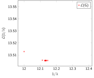
Quisim model:

Model codeOpen in Quisim

Steering { id: steering0; duration:10000; editions:20; x:468; y:43 }
BrentOptimize { id: function0; y:24; x:22; height:181; init:12; lower:12; upper:13; width:283 }
Number { id: number0; x:374; y:163; label:"zᵢ" }
Wire { from: function0.measures[0]; to: number0.parameterValue }
Report { id: statistics2; x:19; y:266; label:"1/λ" }
Wire { from: function0.measures[1]; to: statistics2.parameters[0] }
Report { id: statistics1; x:253; y:266; label:"costs" }
Wire { from: function0.measures[1]; to: rnd0.parameterMean }
RandomExponential { id:rnd0; seed:88; y:529; x:59 }
RandomExponential { id:rnd1; mean:100; seed:143; x:372; y:518 }
Wire { from:rnd0.measureRandomVariate; to:arrive0.parameterDuration }
Wire { from:rnd1.measureRandomVariate; to:perform0.parameterDuration }
Arrive { id:arrive0; x:157; y:532 }
Pipe { from:arrive0.outlet; to:queue0.inlet }
Queue { id:queue0; x:253; y:532 }
Wire { from: function0.measures[1]; to: function1.parameters[0] }
Pipe { from:queue0.outlet; to:perform0.inlet }
Perform { id:perform0; capacity:10; x:490; y:516 }
Pipe { from:perform0.outlet; to:leave0.inlet }
Leave { id:leave0; x:586; y:534 }
Wire { from: queue0.measureLoad; to: statistics0.parameters[0] }
Statistics { id: statistics0; x:480; y:266; timeAverage:true; label:"queue length" }
Function { id: function1; numParameters:2; x:549; y:161; code:"M[0]=P[0]+P[1]"; width:104 }
Wire { from: function1.measures[0]; to: statistics1.parameters[0] }
Wire { from: function1.measures[0]; to: function0.parameters[0] }
Wire { from: statistics0.measures[0]; to: function1.parameters[1] }

---

Job Shop Production

In a job shop, each job has its own routing sequence through machines. The key technique is storing and reading the job-specific sequence using entity attributes.

Guetzli Bakery Example

Scenario: Individualized cookies (Guetzli) with exactly four layers. For each tray:

1. A layer sequence is randomly chosen (e.g., [1, 2, 0] — Caramel, Dough, done)
2. The tray visits each machine in the sequence order
3. After all layers are applied, the tray is baked in the oven

Each tray is a job. The job's routing is stored in entity attributes:

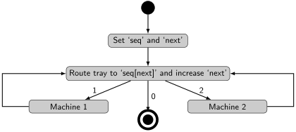
• seq — array of machine indices (0 = done / bake), e.g., [1, 2, 0]
• next — current position in the sequence (starts at 0)

Routing Logic

At each routing decision point:

1. Read seq[next] using Get blocks for both seq and next
2. A Function block evaluates M[0] = P[1][P[0]] (index into the sequence array)
3. The Decide block routes to machine 0, 1, or 2 (where 0 = Bake)
4. After passing through a machine, next is incremented by 1 and the entity returns to the routing decision point

Quisim model:

Model codeOpen in Quisim

RandomUniform { id: randomuniform1; upper:3; x:19; y:142; lower:1 }
Wire { from: randomuniform1.measureRandomVariate; to: function0.parameters[1] }
RandomUniform { id: randomuniform0; upper:3; x:19; y:24; lower:1 }
Wire { from: randomuniform0.measureRandomVariate; to: function0.parameters[0] }
Function { id: function0; numParameters:2; code:"M[0]=[Math.floor(P[0]),Math.floor(P[1]),0]"; x:152; y:153 }
Arrive { id: arrive0; x:192; y:249 }
Set { id: set0; attribute:'seq'; x:352; y:242 }
Pipe { from: arrive0.outlet; to: set0.inlet }
Wire { from: function0.measures[0]; to: set0.parameterValue }
Set { id: set1; value:0; attribute:'next'; x:476; y:242 }
Pipe { from: set0.outlet; to: set1.inlet }
Perform { id: delivery; duration:0; label:'Start'; x:600; y:242 }
Pipe { from: set1.outlet; to: delivery.inlet }
Pipe { from: delivery.outlet; to: get0.inlet }
Get { id: get0; attribute:'seq'; x:724; y:249 }
Wire { from: get0.measureValue; to: function1.parameters[1] }
Get { id: get1; attribute:'next'; x:848; y:249 }
Wire { from: get1.measureValue; to: function1.parameters[0] }
Wire { from: get1.measureValue; to: function2.parameters[0] }
Pipe { from: get0.outlet; to: get1.inlet }
Function { id: function2; code:"M[0]=P[0]+1"; label:'Function++'; x:969; y:314 }
Wire { from: function2.measures[0]; to: set2.parameterValue }
Set { id: set2; attribute:'next'; x:1169; y:293 }
Pipe { from: set2.outlet; to: decide0.inlet }
Function { id: function1; numParameters:2; code:"M[0]=P[1][P[0]]"; x:969; y:170 }
Wire { from: function1.measures[0]; to: decide0.parameters[0] }
Decide { id: decide0; numOutlets:3; x:1293; y:300 }
Pipe { from: get1.outlet; to: set2.inlet; bend:32 }
Queue { id: queue0; y:150; x:1417 }
Pipe { from: decide0.outlets[1]; to: queue0.inlet }
Perform { id: perform0; y:150; x:1542 }
Pipe { from: queue0.outlet; to: perform0.inlet }
Pipe { from: perform0.outlet; to: get0.inlet; bend:-120 }
Queue { id: queue1; y:278; x:1417 }
Pipe { from: decide0.outlets[2]; to: queue1.inlet }
Perform { id: perform1; y:278; x:1542 }
Pipe { from: queue1.outlet; to: perform1.inlet }
Pipe { from: perform1.outlet; to: get0.inlet; bend:-120 }
Pipe { from: decide0.outlets[0]; to: perform4.inlet }
Perform { id: perform4; label:"Bake"; x:1417; y:24; capacity:Infinity }
Pipe { from: perform4.outlet; to: leave0.inlet }
Queue { id: leave0; label:'Finished'; x:1542; y:24 }